# What and Why

Clustering is an unsupervised learning technique. (which is used when you have unlabeled data).
* It is the task of grouping together a set of objects in a way that objects in the same cluster are more similar to each other than to objects in other clusters.
* Similarity is an amount that reflects the strength of relationship between two data objects.

Clustering can be categorized as:
* hard clustering techniques where each element must belong to a single cluster
* soft clustering (or fuzzy clustering) is based on a membership score that defines how much the elements are "compatible" with each cluster
> Apple watch 屬於 3C, 時尚, 鐘錶？

# K-Means

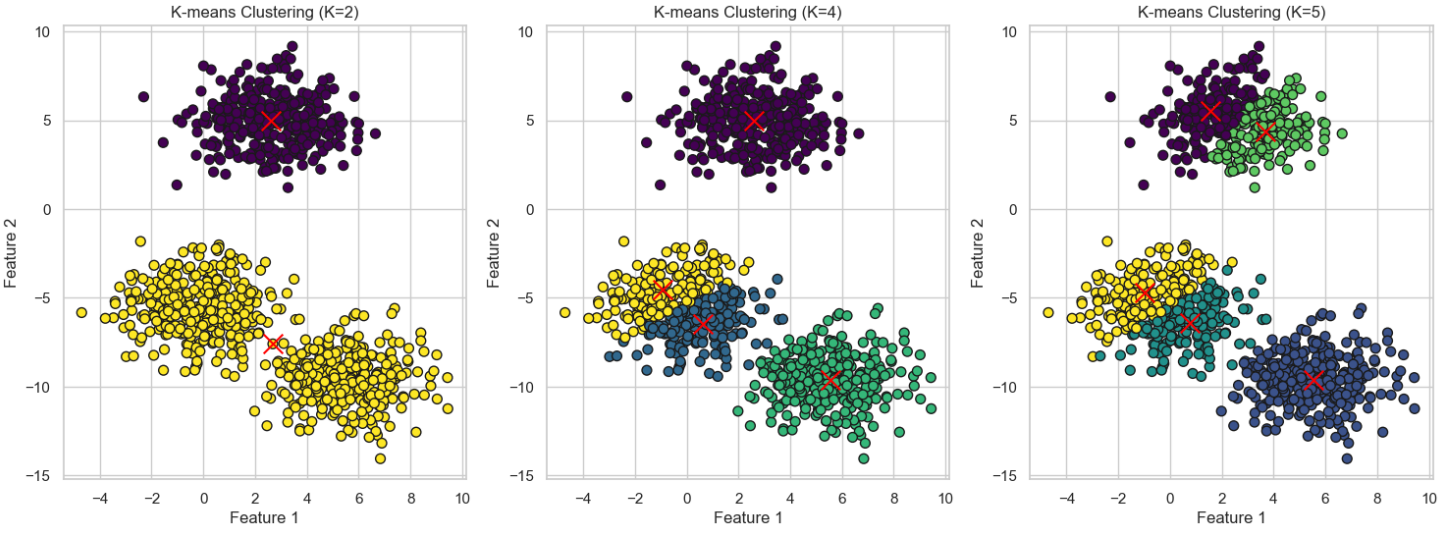
* The goal of this algorithm is to find groups in the data, with the number of groups represented by the variable K.
* The Κ-means clustering algorithm uses iterative refinement to produce a final result.

The process of K-Means works as follows:

1. Decide the Value of K (Number of Clusters):
> Determine the number of clusters　𝐾　you want to create. This is often done based on prior knowledge, experimentation, or methods like the elbow method.
2. Randomly Initialize K Centroids:
> Randomly select　𝐾　points in the data space to serve as the initial centroids (cluster centers).
3. Assign Samples to the Nearest Centroid:
> For each sample in the dataset, calculate the distance between the sample and each of the 　𝐾　centroids.
> Assign the sample to the cluster whose centroid is the closest.
4. Update Centroids:
> For each cluster, compute the new centroid by taking the average of all the samples assigned to that cluster. This new centroid becomes the center of the cluster.
5. Repeat Steps 3 and 4:
> Reassign each sample to the nearest centroid and update the centroids again.
> Repeat this process until the centroids stabilize, meaning they no longer change significantly between iterations, indicating that the algorithm has converged.

import matplotlib.pyplot as plt
import seaborn as sns
from sklearn.datasets import load_iris
from sklearn.cluster import KMeans
from sklearn.decomposition import PCA

# Load the Iris dataset
iris = load_iris()
data = iris.data

# Use PCA to reduce the dimensionality of the data to 2D for visualization
pca = PCA(n_components=2)
reduced_data = pca.fit_transform(data)

# Apply KMeans clustering
kmeans = KMeans(n_clusters=3, random_state=42)
clusters = kmeans.fit_predict(reduced_data)

# Get cluster centers
centers = kmeans.cluster_centers_

# Set plot style
sns.set(style="whitegrid")

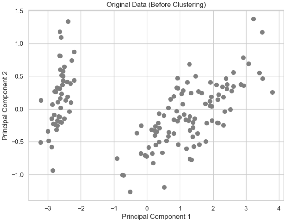
# Visualize the original data (before clustering)
plt.figure(figsize=(8, 6))
plt.scatter(reduced_data[:, 0], reduced_data[:, 1], c='grey', s=50)
plt.title('Original Data (Before Clustering)')
plt.xlabel('Principal Component 1')
plt.ylabel('Principal Component 2')
plt.show()

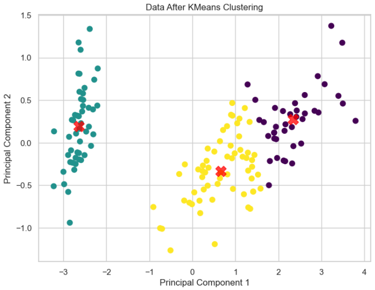
# Visualize the data after applying KMeans clustering with cluster centers
plt.figure(figsize=(8, 6))
plt.scatter(reduced_data[:, 0], reduced_data[:, 1], c=clusters, s=50, cmap='viridis')
plt.scatter(centers[:, 0], centers[:, 1], c='red', s=200, alpha=0.75, marker='X')  # Plot cluster centers
plt.title('Data After KMeans Clustering')
plt.xlabel('Principal Component 1')
plt.ylabel('Principal Component 2')
plt.show()


# K-Means++
1. Select the First Centroid Randomly:
> The first centroid is chosen randomly from the dataset. This is similar to the standard K-means initialization.
2. Calculate Distances:
> For each data point in the dataset, compute its distance from the nearest centroid that has already been chosen. Initially, this will be the distance from the first randomly selected centroid.
3. Select the Next Centroid:
> The next centroid is selected from the data points, with a higher probability given to points that are farther away from the nearest existing centroid. In other words, data points that are far from the already chosen centroids are more likely to be selected as the next centroid. This ensures that centroids are spread out and not clustered together.
4. Repeat Until K Centroids are Chosen:
> Steps 2 and 3 are repeated until all k centroids are selected.


* Initialization: K-means++ improves the initialization process by selecting the first centroid randomly and then choosing subsequent centroids in a way that maximizes the spread between them. Specifically, each new centroid is chosen with a probability proportional to its distance from the nearest previously selected centroid.
* Impact: This smarter initialization helps the algorithm converge faster and often leads to better clustering results. By ensuring that the centroids are well-spread out, K-means++ reduces the likelihood of poor clustering and minimizes the chances of converging to a local minimum.

K-means is based on Euclidean distance, which is radial, and therefore the clusters are expected to be convex
When the data is not convex, the problem cannot be solve using clustering algorithm.

# Choosing K
To find the number of clusters in the data, the user needs to run the K-means clustering algorithm for a range of K values and compare the results.

In general, there is no method for determining exact value of K, but an accurate estimate can be obtained using the following techniques.

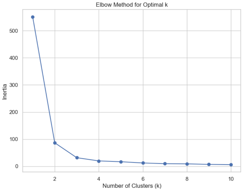
One of the metrics that is commonly used to compare results across different values of K is the mean distance between data points and their cluster centroid.

* mean distance to the centroid as a function of K is plotted and the "**elbow point**" where the rate of decrease sharply shifts, can be used to roughly determine K.
* A number of other techniques exist for validating K, including cross-validation, information criteria, the information theoretic jump method, the silhouette method, and the G-means algorithm.

In addition, monitoring the distribution of data points across groups provides insight into how the algorithm is splitting the data for each K.

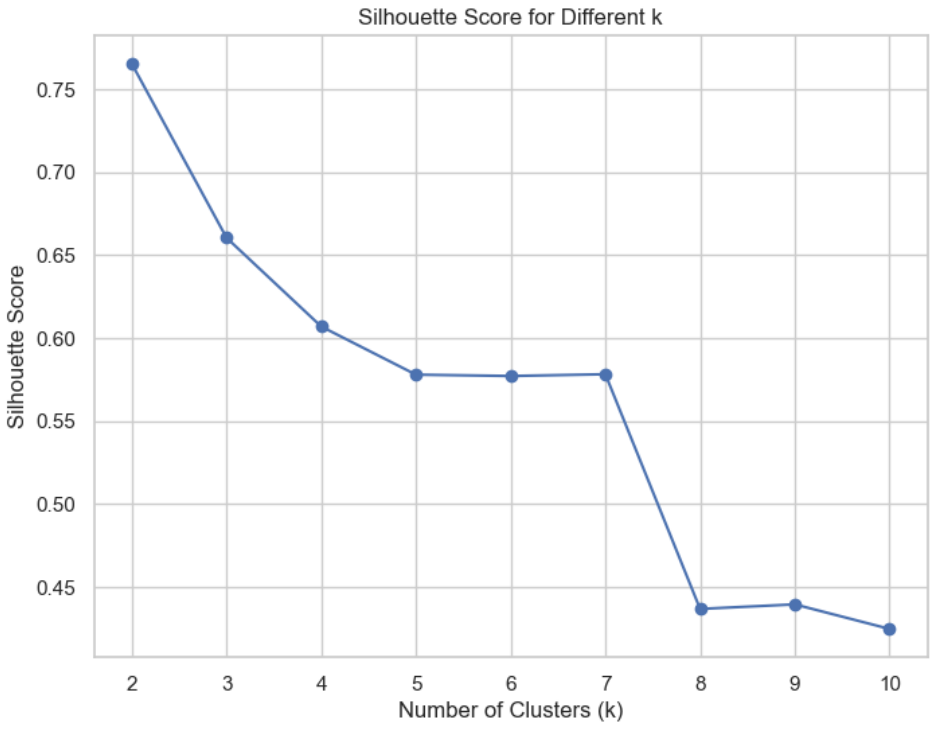
## Silhouette score
The silhouette score is based on the principle of "**maximum internal cohesion and maximum cluster separation**".

In this way, every cluster will contain very similar elements and, selecting two elements belonging to different clusters, their distance should be greater than the maximum intracluster one.

This value is bounded between -1 and 1, with the following interpretation:
A value close to 1 is good (1 is the best condition) because it means that a(xi) ≪ b(xi)
A value close to 0 means that the difference between intra and inter cluster measures is almost null and therefore there's a cluster overlap.
A value close to -1 means that the sample has been assigned to a wrong cluster because a(xi) ≫ b(xi)

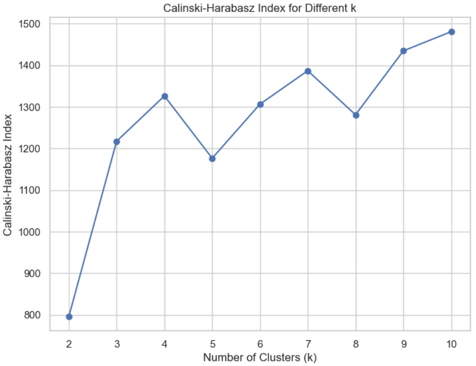
## Calinski-Harabasz index
Also based on the concept of dense and well-separated clusters

If the ground truth labels are not known, the Calinski-Harabasz index -- also known as the Variance Ratio Criterion - can be used to evaluate the model, where a higher Calinski-Harabasz score relates to a model with better defined clusters

## DBSCAN
DBSCAN is a powerful algorithm that can easily solve non-convex problems where k-means fails.
The DBSCAN algorithm should be used to find associations and structures in data that are hard to find manually but that can be relevant and useful to find patterns and predict trends.

The procedure starts by analyzing a small area (formally, a point surrounded by a minimum number of other samples). If the density is enough, it is considered part of a cluster.
At this point, the neighbors are taken into account. If they also have a high density, they are merged with the first area; otherwise, they determine a topological separation.
When all the areas have been scanned, the clusters have also been determined because they are islands surrounded by empty space.

The DBSCAN algorithm basically requires 2 parameters:
> **minPoints**: the minimum number of points to form a dense region. For example, if we set the minPoints parameter as 5, then we need at least 5 points to form a dense region.
> **eps**: the minimum distance between two points. It means that if the distance between two points is lower or equal to this value (eps), these points are considered neighbors.

DBSCAN會依據data性質自行決定最終Cluster的數量

import matplotlib.pyplot as plt
import seaborn as sns
from sklearn.cluster import KMeans, DBSCAN
from sklearn.metrics import silhouette_score, calinski_harabasz_score
from sklearn.datasets import load_iris
import pandas as pd

# Load the Iris dataset
iris = load_iris()
df = pd.DataFrame(data=iris.data, columns=iris.feature_names)

# Use petal length and petal width for clustering
x = df[['petal length (cm)', 'petal width (cm)']]

# Elbow method (using inertia)
DistanceList = []
for i in range(1, 11):  # Test different numbers of clusters from 1 to 10
    KM = KMeans(n_clusters=i, n_init='auto', random_state=1)
    KM.fit(x)
    DistanceList.append(KM.inertia_)  # Record inertia (sum of squared distances to centroids)

plt.figure(figsize=(8, 6))
plt.plot(range(1, 11), DistanceList, marker='o')
plt.title('Elbow Method for Optimal k')
plt.xlabel('Number of Clusters (k)')
plt.ylabel('Inertia')
plt.show()


# Silhouette Score and Calinski-Harabasz Index for different k
silhouette_scores = []
calinski_harabasz_scores = []

for i in range(2, 11):  # Silhouette and Calinski-Harabasz can't be calculated for k=1
    KM = KMeans(n_clusters=i, n_init='auto', random_state=1)
    clusters = KM.fit_predict(x)
    
    # Calculate Silhouette score
    silhouette_avg = silhouette_score(x, clusters)
    silhouette_scores.append(silhouette_avg)
    
    # Calculate Calinski-Harabasz index
    calinski_harabasz_avg = calinski_harabasz_score(x, clusters)
    calinski_harabasz_scores.append(calinski_harabasz_avg)

# Plot Silhouette Score
plt.figure(figsize=(8, 6))
plt.plot(range(2, 11), silhouette_scores, marker='o', label='Silhouette Score')
plt.title('Silhouette Score for Different k')
plt.xlabel('Number of Clusters (k)')
plt.ylabel('Silhouette Score')
plt.show()


# Plot Calinski-Harabasz Index
plt.figure(figsize=(8, 6))
plt.plot(range(2, 11), calinski_harabasz_scores, marker='o', label='Calinski-Harabasz Index')
plt.title('Calinski-Harabasz Index for Different k')
plt.xlabel('Number of Clusters (k)')
plt.ylabel('Calinski-Harabasz Index')
plt.show()


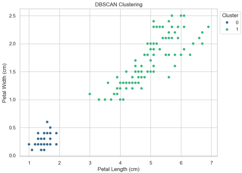
# DBSCAN
dbscan = DBSCAN(eps=0.5, min_samples=5)
dbscan_clusters = dbscan.fit_predict(x)

# Visualize DBSCAN result
plt.figure(figsize=(8, 6))
sns.scatterplot(x='petal length (cm)', y='petal width (cm)', data=df, hue=dbscan_clusters, palette='viridis')
plt.title('DBSCAN Clustering')
plt.xlabel('Petal Length (cm)')
plt.ylabel('Petal Width (cm)')
plt.legend(title='Cluster', loc='upper left', bbox_to_anchor=(1, 1))
plt.show()