Strong learners:

* trained models on single instances,iterating an algorithm in order to minimize a target loss function
* this approach is based on so-called strong learners, or methods that are optimized to solve a specific problem by looking for the best possible solution

Weak learners:

* this approach is based on a set of weak learners that can be trained in parallel or sequentially and used as an ensemble based on a majority vote or the averaging of results.
* an ensemble is just a collection of models which come together(e.g. mean of all predictions) to give a final prediction
* one important point is that our choice of base models should be coherent with the way we aggregate these models.

if we choose base models with low bias but high variance[ie. complex models such as neural networks], it should be with an aggregating method that tends to reduce variance

if we choose base models with low variance but high bias[ie. simple models such as Linear regression], it should be with an aggregating method that tends to reduce bias.

平均或加權平均通過平滑多個高方差模型的預測結果，減少了預測中的隨機波動，從而降低了方差。
多數投票通過集成多個高偏差模型的預測結果，糾正了單個模型的錯誤預測，從而降低了偏差。

Three popular techniques:
Max voting(使用了 VotingClassifier 並設置 voting='hard')
Averaging (使用了 VotingClassifier 並設置 voting='soft')
Weighted average: on can assign weights to different models.

# Import necessary libraries
from sklearn.datasets import load_breast_cancer
from sklearn.model_selection import train_test_split
from sklearn import preprocessing
from sklearn.ensemble import VotingClassifier
from sklearn.linear_model import LogisticRegression
from sklearn.naive_bayes import GaussianNB
from sklearn.svm import SVC
from sklearn.metrics import accuracy_score

# Load the breast cancer dataset
data = load_breast_cancer(as_frame=True)

# Split the dataset into training and testing sets
X_train, X_test, y_train, y_test = train_test_split(data['data'], data['target'], test_size=0.2, random_state=100)

# Preprocess the data
scaler = preprocessing.StandardScaler().fit(X_train)
X_train = scaler.transform(X_train)
X_test = scaler.transform(X_test)

lr = LogisticRegression().fit(X_train, y_train)
lr_score = lr.score(X_test, y_test)
print(f'Logistic Regression accuracy: {lr_score:.4f}')

gnb = GaussianNB().fit(X_train, y_train)
gnb_score = gnb.score(X_test, y_test)
print(f'Naive Bayes accuracy: {gnb_score:.4f}')

svc = SVC(probability=True).fit(X_train, y_train)
svc_score = svc.score(X_test, y_test)
print(f'Support Vector Machine accuracy: {svc_score:.4f}')

Logistic Regression accuracy: 0.9737
Naive Bayes accuracy: 0.9386
Support Vector Machine accuracy: 0.9649

# Define the base models
log_clf = LogisticRegression()
nb_clf = GaussianNB()
svc_clf = SVC(probability=True)  # Set probability=True for soft voting

# Create the VotingClassifier with hard voting
voting_clf_hard = VotingClassifier(
    estimators=[
        ('lr', log_clf),
        ('nb', nb_clf),
        ('svc', svc_clf)
    ],
    voting='hard'
)

voting_clf_hard.fit(X_train, y_train)
voting_clf_hard_score = voting_clf_hard.score(X_test, y_test)
print(f'Voting Classifier (hard) accuracy: {voting_clf_hard_score:.4f}')

# Create the VotingClassifier with soft voting
voting_clf_soft = VotingClassifier(
    estimators=[
        ('lr', log_clf),
        ('nb', nb_clf),
        ('svc', svc_clf)
    ],
    voting='soft'
)

voting_clf_soft.fit(X_train, y_train)
voting_clf_soft_score = voting_clf_soft.score(X_test, y_test)
print(f'Voting Classifier (soft) accuracy: {voting_clf_soft_score:.4f}')

# Create the VotingClassifier with weighted soft voting
voting_clf_weighted = VotingClassifier(
    estimators=[
        ('lr', log_clf),
        ('nb', nb_clf),
        ('svc', svc_clf)
    ],
    voting='soft',
    weights=[2, 1, 3]  # Example weights for the classifiers
)

voting_clf_weighted.fit(X_train, y_train)
voting_clf_weighted_score = voting_clf_weighted.score(X_test, y_test)
print(f'Voting Classifier (weighted soft) accuracy: {voting_clf_weighted_score:.4f}')

Voting Classifier (hard) accuracy: 0.9649
Voting Classifier (soft) accuracy: 0.9561
Voting Classifier (weighted soft) accuracy: 0.9737

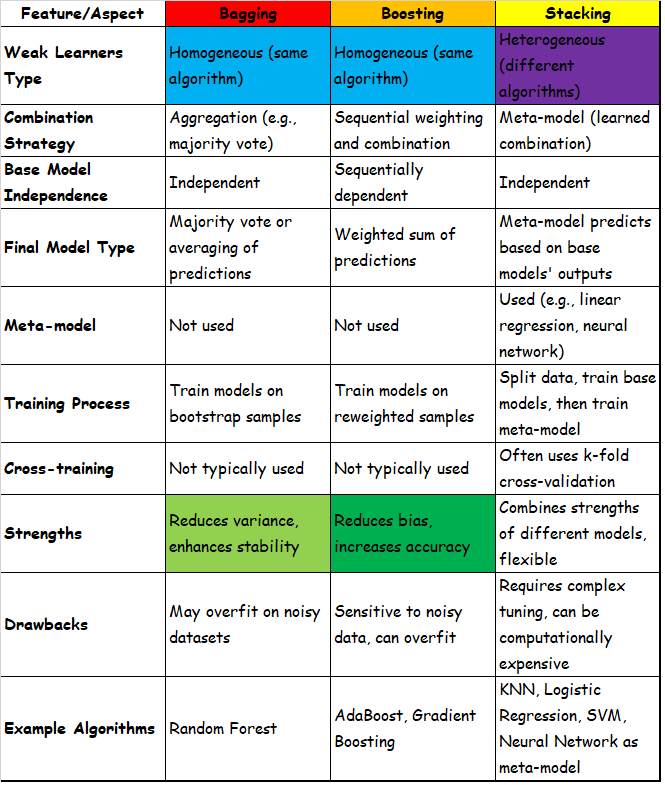
# Bagging

## Steps:

1. Random Sampling (Bootstrapping):
Create random subsets from the original dataset through bootstrapping (sampling with replacement).
3. Feature Selection:
Each subset includes all features (some algorithms might include randomly selected features).
5. Training Base Models:
Use a user-specified base estimator to train on each of these smaller sets. Usually, only one type of base estimator is used.(Ex. SVM -> ALL)
7. Combining Predictions:
Combine the predictions from each model to get the final result. Combination methods can be weighted average, majority vote, or normal average.

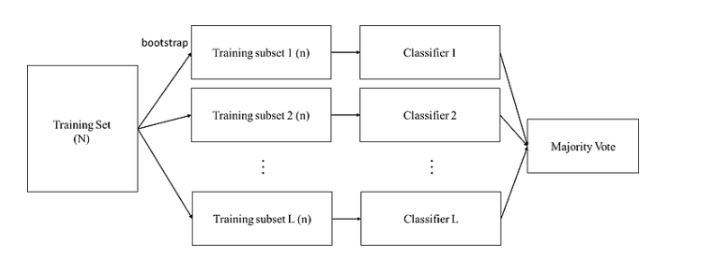
## Techniques:
* Often uses homogeneous weak learners (e.g., multiple decision trees).
* The main goal is to **reduce the variance of the model**, making the ensemble model's predictions more stable.
* Constructs many independent predictors/models/learners and combines their predictions using some model averaging techniques (e.g., weighted average, majority vote, or normal average).
* Since the models are independent, they can be trained in parallel.

Bagging的優點在於原始訓練樣本中有噪聲資料(不好的資料)，透過Bagging抽樣就有機會不讓有噪聲資料被訓練到，所以可以降低模型的不穩定性

import numpy as np
import matplotlib.pyplot as plt
from sklearn.datasets import load_breast_cancer
from sklearn.ensemble import BaggingClassifier, RandomForestClassifier
from sklearn.model_selection import train_test_split
from sklearn.metrics import accuracy_score, confusion_matrix, ConfusionMatrixDisplay

# 載入Breast Cancer資料集
data = load_breast_cancer()
X, y = data.data, data.target

# 分割資料成訓練集和測試集
X_train, X_test, y_train, y_test = train_test_split(X, y, test_size=0.3, random_state=42)

# 使用Bagging來訓練隨機森林模型
bagging_clf = BaggingClassifier(
    estimator=RandomForestClassifier(n_estimators=100),
    n_estimators=10,
    random_state=42
)
bagging_clf.fit(X_train, y_train)

# 預測測試集
y_pred = bagging_clf.predict(X_test)

# 計算準確率
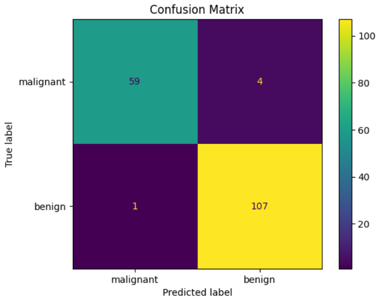
accuracy = accuracy_score(y_test, y_pred)
print(f'Accuracy: {accuracy:.2f}')

# 混淆矩陣
cm = confusion_matrix(y_test, y_pred)
disp = ConfusionMatrixDisplay(confusion_matrix=cm, display_labels=data.target_names)
disp.plot()

# 顯示圖表
plt.title('Confusion Matrix')
plt.show()


import numpy as np
from sklearn.datasets import load_breast_cancer
from sklearn.ensemble import BaggingClassifier
from sklearn.linear_model import LogisticRegression
from sklearn.naive_bayes import GaussianNB
from sklearn.svm import SVC
from sklearn.model_selection import train_test_split
from sklearn.metrics import accuracy_score

# 載入Breast Cancer資料集
data = load_breast_cancer()
X, y = data.data, data.target

# 分割資料成訓練集和測試集
X_train, X_test, y_train, y_test = train_test_split(X, y, test_size=0.2, random_state=42)

# 定義分類器
classifiers = {
    "Logistic Regression": LogisticRegression(max_iter=10000),
    "Gaussian NB": GaussianNB(),
    "SVM": SVC(probability=True)
}

# 訓練並評估每個分類器
for name, clf in classifiers.items():
    bagging_clf = BaggingClassifier(
        estimator=clf,
        n_estimators=100,
        random_state=42
    )
    bagging_clf.fit(X_train, y_train)
    
    # 預測測試集
    y_pred = bagging_clf.predict(X_test)
    
    # 計算準確率
    accuracy = accuracy_score(y_test, y_pred)
    print(f'{name} Accuracy with Bagging: {accuracy:.2f}')
    
    # 訓練原始分類器（不使用Bagging）並進行評估
    clf.fit(X_train, y_train)
    y_pred_original = clf.predict(X_test)
    accuracy_original = accuracy_score(y_test, y_pred_original)
    print(f'{name} Accuracy without Bagging: {accuracy_original:.2f}')
    print('-' * 50)

Logistic Regression Accuracy with Bagging: 0.96
Logistic Regression Accuracy without Bagging: 0.96
Gaussian NB Accuracy with Bagging: 0.97
Gaussian NB Accuracy without Bagging: 0.97
SVM Accuracy with Bagging: 0.95
SVM Accuracy without Bagging: 0.95

> Logistic Regression：
> 模型特性：Logistic Regression 是一個中等複雜度的模型，偏差和方差都處於中等水平。
> 結果分析：使用 Bagging 前後的準確率均為 0.96，這表明在這個數據集上，Bagging 對 Logistic Regression 的效果不顯著。這可能是因為 Logistic Regression 已經在這個問題上表現得很好，其原本的偏差和方差已經較為平衡，Bagging 並未能顯著改善其性能。
> Gaussian NB：
> 模型特性：Gaussian NB 是一個簡單的模型，通常具有低方差和高偏差。
> 結果分析：使用 Bagging 前後的準確率均為 0.97，這表明在這個數據集上，Bagging 對 Gaussian NB 的效果也不顯著。這符合預期，因為 Gaussian NB 的方差已經很低，Bagging 難以進一步降低其方差。
> SVM：
> 模型特性：SVM 是一個複雜的模型，通常具有高方差和低偏差。
> 結果分析：使用 Bagging 前後的準確率均為 0.95，這表明在這個數據集上，Bagging 對 SVM 的效果同樣不顯著。這可能是因為這個數據集並沒有讓 SVM 過擬合，或者 SVM 本身已經有較好的正則化（例如使用了適當的C參數），因此 Bagging 沒有顯著改進其性能。

# Boosting

Boosting is an ensemble technique in which the predictors are not made independently, but sequentially.
* this technique employs the logic which the subsequent predictors learn from the mistakes of the previous predictors.
* the predictors can be chosen from a range of models like decision trees, regressors, classifiers etc.
* examples of bosting are adaboost, gredient boosting, and XGBoost.


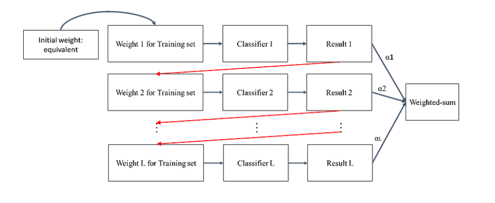
Boosting的關鍵在於針對舊分類器的錯誤樣本提高其權重，然後訓練新的分類器。這樣，新分類器會更關注這些被錯誤分類的樣本特徵，從而提高整體分類的準確性。

由於Boosting將注意力集中在分類錯誤的資料上，因此Boosting對訓練資料的噪聲非常敏感，如果一筆訓練資料噪聲資料很多，那後面分類器都會集中在進行噪聲資料上分類，反而會影響最終的分類性能。

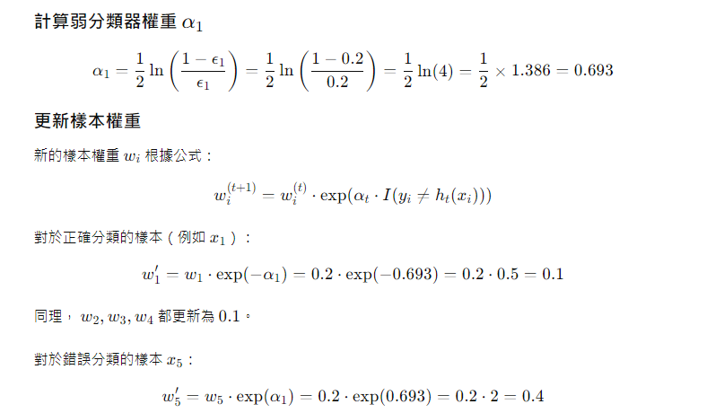
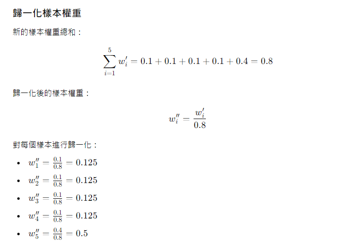
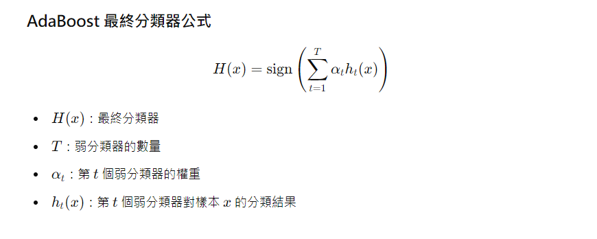
對於Boosting來說，有兩個關鍵，一是在**如何改變訓練資料的權重**；二是**如何將多個弱分類器組合成一個強分類器**。而且存在一個重大的缺陷：該分類算法要求預先知道弱分類器識別準確率的下限。

解決方法：
* 使用基於剪枝（pruning）的弱分類器：例如，決策樹中可以使用深度限制或葉節點樣本數限制來防止過擬合噪聲數據。
* 引入正則化：在弱分類器的訓練過程中引入正則化項，防止過度關注噪聲樣本。
* 早停法（Early Stopping）：在 Boosting 過程中監控性能指標，當發現性能不再提高甚至下降時停止添加新的弱分類器。
* 使用穩健的損失函數：如在 AdaBoost 的基礎上使用更穩健的損失函數（例如 Logistic Loss）來減少對噪聲數據的敏感度。

## AdaBoost

Adaboost is short for adaptive boosting
* the dataset used for training is continuously adapted to frorce the model to focus on those samples that are misclassified.
* moreover, the classifiers are added sequentially, so a new one boosts the previous one by improving the performance in those areas where it was not as accurate as expected.

Pseudocode of AdaBoost:
1. initially set uniform example weights.
for each base learner do:
1. train base learner with a weighted sample.
1. test base learner on all data.
1. set learner weight with a weighted error.
1. set example weights based on ensemble predictions
end for

Math Exaple:



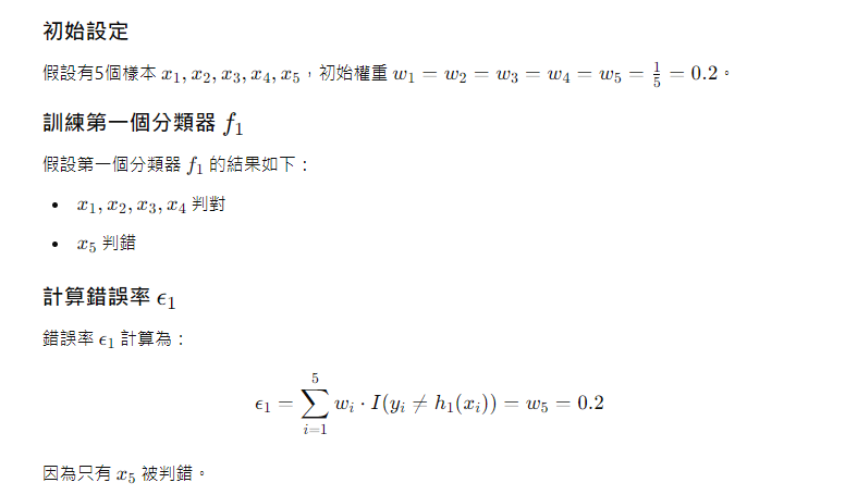
假設T=2



對於𝑥1​：
𝐻(𝑥1)=sign(0.693×1+0.5493×1)=sign(0.693+0.5493)=sign(1.2423)=1
對於𝑥2​：
𝐻(𝑥2)=sign(0.693×1+0.5493×(−1))=sign(0.693−0.5493)=sign(0.1437)=1
對於𝑥3 ：
𝐻(𝑥3)=sign(0.693×1+0.5493×1)=sign(0.693+0.5493)=sign(1.2423)=1
對於𝑥4​：
𝐻(𝑥4)=sign(0.693×1+0.5493×(−1))=sign(0.693−0.5493)=sign(0.1437)=1
對於𝑥5​：
𝐻(𝑥5)=sign(0.693×(−1)+0.5493×1)=sign(−0.693+0.5493)=sign(−0.1437)=−1

第一個分類器預測的五個結果是[1,1,1,1,-1]
第二的分類器預測的五個結果是[1,-1,1,-1,1]
最後兩個分類器合成五個結果是[1,1,1,1,-1]

from sklearn.datasets import load_breast_cancer
from sklearn.model_selection import train_test_split, GridSearchCV
from sklearn.ensemble import AdaBoostClassifier
from sklearn.tree import DecisionTreeClassifier
from sklearn.metrics import accuracy_score

# 加載資料集
data = load_breast_cancer()
X = data.data
y = data.target

# 切分訓練集和測試集
X_train, X_test, y_train, y_test = train_test_split(X, y, test_size=0.2, random_state=42)

# 初始化基分類器
base_clf = DecisionTreeClassifier(max_depth=1)

# 初始化 AdaBoost 分類器
ada_clf = AdaBoostClassifier(
    estimator=base_clf,
    n_estimators=50,
    random_state=42
)

# 設置網格搜索的參數範圍
param_grid = {
    'learning_rate': [0.01, 0.1, 0.5, 1.0, 1.5, 2.0]
}

# 使用網格搜索和交叉驗證來尋找最佳參數
grid_search = GridSearchCV(ada_clf, param_grid, cv=5, scoring='accuracy')
grid_search.fit(X_train, y_train)

# 打印最佳參數
print("Best parameters found: ", grid_search.best_params_)

# 使用最佳參數訓練模型
best_ada_clf = grid_search.best_estimator_
best_ada_clf.fit(X_train, y_train)

# 預測測試集
y_pred = best_ada_clf.predict(X_test)

# 計算準確率
accuracy = accuracy_score(y_test, y_pred)
print(f'Accuracy: {accuracy:.4f}')

Best parameters found: {'learning_rate': 1.0}
Accuracy: 0.9737

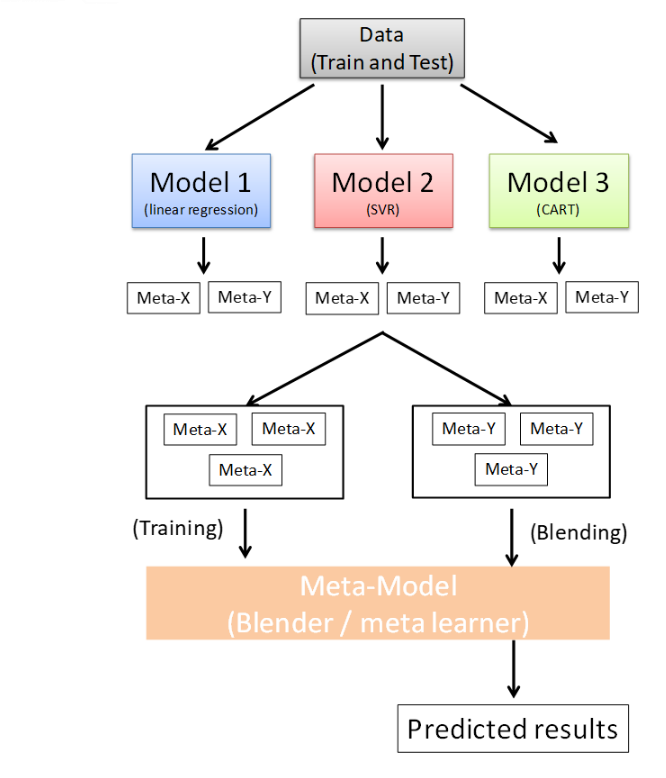
# Stacking

Stacking mainly differ form bagging and boosting on two points.
* stacking often considers **heterogeneous weak learners**(different learning algorithms are combined) whereas bagging and boosting consider mainly homogeneous weak learners.
* stacking learns to combine the base models using a meta-model whereas bagging and boosting combine weak learners following deterministic algorithms.
the meta-model is often simple, providing a smooth interpretation of the predictions made by the base models. As such, linear models are often used as the meta-model .

For example, for a classification problem,we can choose weak learners as a KNN classifier, a logistic regression and a SVM, and decide to learn a neural newtowk as meta-model.
then, the neural network will take as inputs the outputs of our three weak learners and will learn to return final predictions based on it.


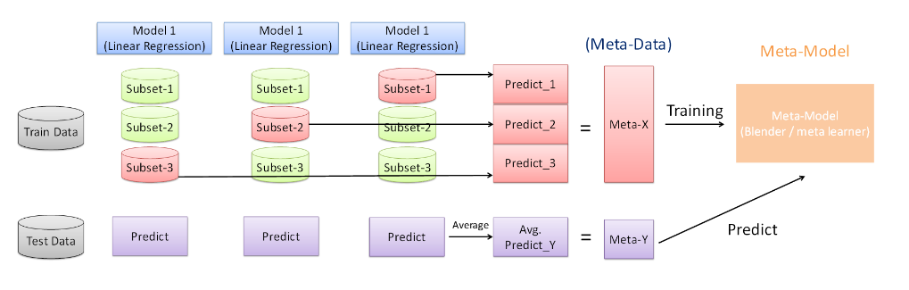
Assume that we want to fit a stacking ensemble composed of L weak learners.
then we have to follow the steps :
* split the training data in two folds
* choose L weak learners and fit them to data of the first fold
* for each of the L weak learners, make predictions for observations in the second fold
* fit the meta-model on the second fold, using predictions made by the weak learners as inputs

An obvious drawback of splitting into half each of our dataset in two parts is that we only have half of the data in two parts is that we only have of the data to train the base models and half of the data to train the meta-model.

in order to overcome this limitation, we can however follow some kind of '**k-fold cross-training**' approach such that all the observations can be used to train the meta-model


import numpy as np
import pandas as pd
from sklearn.datasets import load_breast_cancer
from sklearn.model_selection import train_test_split, KFold
from sklearn.ensemble import AdaBoostRegressor
from sklearn.tree import DecisionTreeRegressor

# Load the dataset
data = load_breast_cancer()
X = data.data
y = data.target

# Split the data into train and test sets
X_train, X_test, y_train, y_test = train_test_split(X, y, test_size=0.2, random_state=42)

# Prepare the 3-fold split
kf = KFold(n_splits=3, shuffle=True, random_state=42)
train_folds = list(kf.split(X_train))

meta_x = []
meta_y = []

# Function to perform stacking and generate meta-features
def stacking_model(model, X_train, y_train, X_test, train_folds):
    meta_x = []
    meta_y = []

    for i, (train_index, valid_index) in enumerate(train_folds):
        X_tr, X_val = X_train[train_index], X_train[valid_index]
        y_tr, y_val = y_train[train_index], y_train[valid_index]

        model.fit(X_tr, y_tr)
        tmp_meta_x = model.predict(X_val)
        tmp_meta_y = model.predict(X_test)
        
        meta_x.extend(tmp_meta_x)
        meta_y.append(tmp_meta_y)
    
    mean_meta_y = np.mean(meta_y, axis=0)
    return np.array(meta_x), mean_meta_y

# First model: Linear Regression
from sklearn.linear_model import LinearRegression
lr = LinearRegression()
meta_x_lr, mean_meta_y_lr = stacking_model(lr, X_train, y_train, X_test, train_folds)

meta_train_1 = pd.DataFrame({'meta_x': meta_x_lr, 'y': y_train})
meta_test_1 = pd.DataFrame({'meta_y': mean_meta_y_lr, 'y': y_test})

# Second model: Support Vector Regression (SVR)
from sklearn.svm import SVR
svr = SVR()
meta_x_svr, mean_meta_y_svr = stacking_model(svr, X_train, y_train, X_test, train_folds)

meta_train_2 = pd.DataFrame({'meta_x': meta_x_svr, 'y': y_train})
meta_test_2 = pd.DataFrame({'meta_y': mean_meta_y_svr, 'y': y_test})

# Third model: Decision Tree Regressor
dtr = DecisionTreeRegressor()
meta_x_dtr, mean_meta_y_dtr = stacking_model(dtr, X_train, y_train, X_test, train_folds)

meta_train_3 = pd.DataFrame({'meta_x': meta_x_dtr, 'y': y_train})
meta_test_3 = pd.DataFrame({'meta_y': mean_meta_y_dtr, 'y': y_test})

# Combine the meta-train datasets
big_meta_train = pd.concat([meta_train_1, meta_train_2, meta_train_3])

# Meta-model with AdaBoost
ada = AdaBoostRegressor(estimator=DecisionTreeRegressor(max_depth=3), n_estimators=100, random_state=42)
ada.fit(big_meta_train['meta_x'].values.reshape(-1, 1), big_meta_train['y'])

# Predict with the meta-test datasets
final_1 = ada.predict(meta_test_1['meta_y'].values.reshape(-1, 1))
final_2 = ada.predict(meta_test_2['meta_y'].values.reshape(-1, 1))
final_3 = ada.predict(meta_test_3['meta_y'].values.reshape(-1, 1))

# Average the predictions and calculate the Mean Squared Error (MSE)
final_y = (final_1 + final_2 + final_3) / 3
mse = np.mean((final_y - y_test) ** 2)

print(f'Mean Squared Error: {mse}')

Mean Squared Error: 0.23255968111869074