# Linear Problems
* Definition:
Linear problems typically involve first-order equations or quadratic equations. In these problems, the objective function is either linear (e.g., 𝑦=𝑎𝑥+𝑏) or a convex quadratic equation (e.g., 𝑦=𝑎𝑥2+𝑏𝑥+𝑐).
* Characteristics:
**First-order functions**: The graph is a straight line, with no minima or maxima.
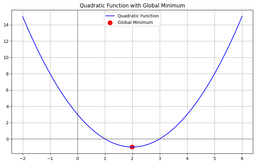
**Quadratic functions**: The graph is a parabola, with a single global minimum (if it opens upwards) or a global maximum (if it opens downwards).
**Global Minimum/Maximum**: The only extremum point in a quadratic function is the global minimum or maximum.

# Nonlinear Problems
* Definition:
Nonlinear problems involve polynomial equations of degree higher than two (e.g., cubic, quartic, etc.), or other more complex functions (e.g., exponential, logarithmic).
* Characteristics:
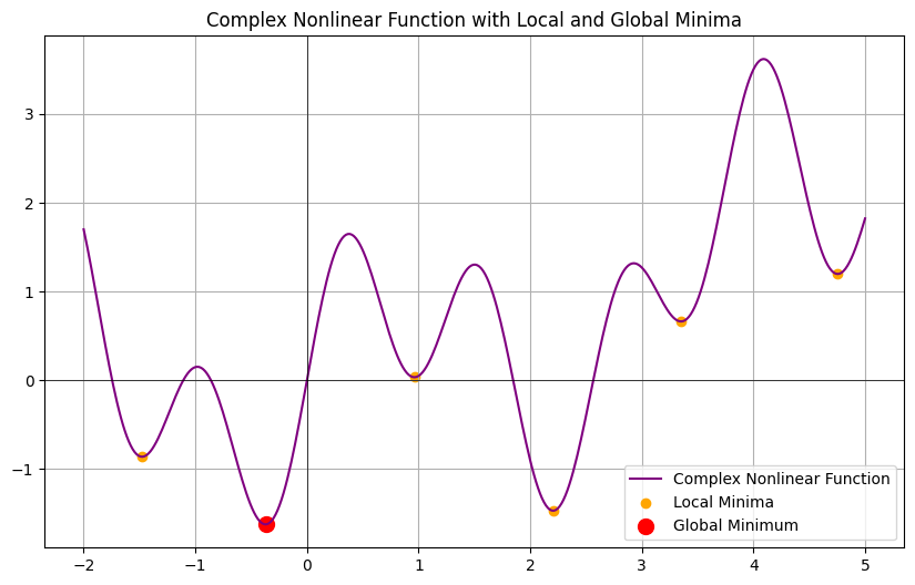
**Multiple extrema**: The graph of a nonlinear problem may have multiple extrema points, including local minima, local maxima, and saddle points.
**Global Minimum**: The lowest point in the entire domain of the function.
**Local Minimum**: The lowest point in a local region, but not necessarily the lowest in the entire domain.

# How to find the Global Minimum and Local Minimum
## Linear Problems (e.g., Quadratic Function)
1. Calculate the first derivative: Set the first derivative 𝑓′(𝑥)=0
1. Find the critical point: Solve for 𝑥 where the first derivative equals zero.
1. Calculate the second derivative: Determine the nature of the critical point.
If 𝑓′′(𝑥)>0, the point is a global minimum.
If 𝑓′′(𝑥)<0, the point is a global maximum.

## Nonlinear Problems

1. Calculate the first derivative: Set the first derivative 𝑓′(𝑥)=0 to find all critical points.
1. Calculate the second derivative: For each critical point 𝑥, compute the second derivative 𝑓′′(𝑥)
* 𝑓′′(𝑥)>0 indicates a local minimum.
* 𝑓′′(𝑥)<0 indicates a local maximum.
1. Compare extrema points: Compare the function values of all local minima to determine the global minimum. Also, consider the behavior of the function at infinity if needed.

**Linear Problems: Typically have only one minimum or maximum, which is the global minimum or maximum.
Nonlinear Problems: May have multiple local minima, requiring comparison to identify the global minimum.**

import numpy as np
import matplotlib.pyplot as plt

# 定義線性問題中的二次函數（簡單的二次函數案例）
def simple_quadratic_function(x):
    return x**2 - 4*x + 3

# 定義x軸範圍
x = np.linspace(-2, 6, 400)

# 計算函數值
y_simple_quadratic = simple_quadratic_function(x)

# 找到二次函數的最小值
# 二次函數的全域極小值和唯一的極小值
global_minimum_index_quadratic = np.argmin(y_simple_quadratic)
global_minimum_x_quadratic = x[global_minimum_index_quadratic]
global_minimum_y_quadratic = y_simple_quadratic[global_minimum_index_quadratic]

# 繪製圖形
plt.figure(figsize=(10, 6))
plt.plot(x, y_simple_quadratic, label='Quadratic Function', color='blue')
plt.scatter(global_minimum_x_quadratic, global_minimum_y_quadratic, color='red', label='Global Minimum', s=100)
plt.title("Quadratic Function with Global Minimum")
plt.axhline(0, color='black',linewidth=0.5)
plt.axvline(0, color='black',linewidth=0.5)
plt.grid(True)
plt.legend()
plt.show()


# 定義更複雜的非線性函數
def complex_nonlinear_function(x):
    return np.sin(5*x) + np.sin(2*x) + 0.1*x**2

# 定義x軸範圍
x = np.linspace(-2, 5, 400)

# 計算函數值
y_complex_nonlinear = complex_nonlinear_function(x)

# 找到函數的全域極小值和局部極小值
# 使用SciPy來尋找最小值點
from scipy.signal import find_peaks

# 找到局部極小值
local_minima_indices = find_peaks(-y_complex_nonlinear)[0]
local_minima_x = x[local_minima_indices]
local_minima_y = y_complex_nonlinear[local_minima_indices]

# 找到全域極小值
global_minimum_index = np.argmin(y_complex_nonlinear)
global_minimum_x = x[global_minimum_index]
global_minimum_y = y_complex_nonlinear[global_minimum_index]

# 繪製圖形
plt.figure(figsize=(10, 6))
plt.plot(x, y_complex_nonlinear, label='Complex Nonlinear Function', color='purple')
plt.scatter(local_minima_x, local_minima_y, color='orange', label='Local Minima')
plt.scatter(global_minimum_x, global_minimum_y, color='red', label='Global Minimum', s=100)
plt.title("Complex Nonlinear Function with Local and Global Minima")
plt.axhline(0, color='black',linewidth=0.5)
plt.axvline(0, color='black',linewidth=0.5)
plt.grid(True)
plt.legend()
plt.show()


Example:

f(x) = x^4^ - x^2^

一次微分f'(x)=4x^3^ - 2x = 0
f'(x) = 0 時可以求出 2x(2x^2^ - 1) = 0 , x = 0 or x = +- 1/2^-1^

二次微分f''(x) = 12x^2^ - 2
帶入x = 0 臨界值時,f''(0) = -2, x=0代表是local maximum
帶入x = +- 1/2^-1^ 臨界值時,f''(+- 1/2^-1^) = 4 > 0, 這代表x = +- 1/2^-1^ 是局部最小值

# Local minimum and a Saddle point
## Local Minimum: All eigenvalues of the Hessian matrix are positive
For example, consider a simple quadratic function of two variables:

𝑓(𝑥,𝑦)=𝑥^2^ + 𝑦^2^
H=[∂^2^f/∂x^2^ , ∂^2^f/∂x∂y , ∂^2^f/∂x∂y , ∂^2^f/∂y^2^]=[2,0,0,2]
The eigenvalues are 2 and 2, both positive, which means the curvature near this point is upward. Therefore, this is a local minimum, and the curve forms an upward bowl (concave up).

## Local Maximum: All eigenvalues of the Hessian matrix are negative
𝑓(𝑥,𝑦)= - 𝑥^2^ - 𝑦^2^
H=[∂^2^f/∂x^2^ , ∂^2^f/∂x∂y , ∂^2^f/∂x∂y , ∂^2^f/∂y^2^]=[-2,0,0,-2]
The eigenvalues are -2 and -2, both negative, which means the curvature near this point is downward. Therefore, this is a local maximum, and the curve forms a downward bowl (convex).

## Saddle Point: The Hessian matrix has both positive and negative eigenvalues
𝑓(𝑥,𝑦)= 𝑥^2^ - 𝑦^2^
H=[∂^2^f/∂x^2^ , ∂^2^f/∂x∂y , ∂^2^f/∂x∂y , ∂^2^f/∂y^2^]=[2,0,0,-2]
The eigenvalues are 2 and -2, one positive and one negative, which means the point has upward curvature in one direction (minimum) and downward curvature in another direction (maximum). This is a saddle point, and the curve forms an upward shape in one direction and downward in another.

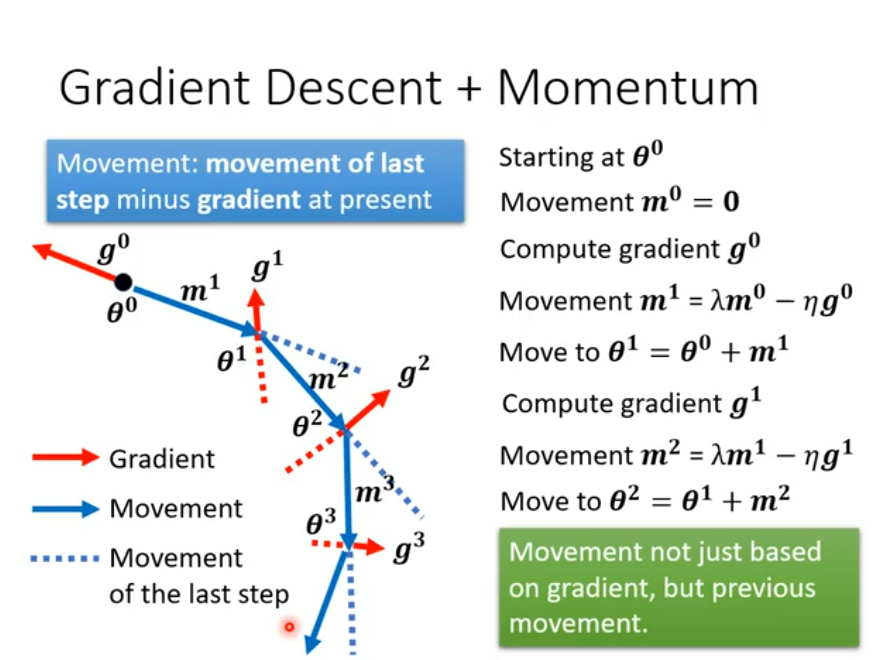
# Momentum

* Faster Convergence: Momentum considers not only the current gradient but also the gradients from previous iterations. This cumulative effect helps speed up the algorithm in directions where the gradient consistently points in the same direction.
* Reducing Oscillations: In gradient updates, the algorithm can sometimes oscillate between directions, especially near minima or when traversing steep valleys. Momentum helps smooth out these oscillations, leading to more stable convergence.


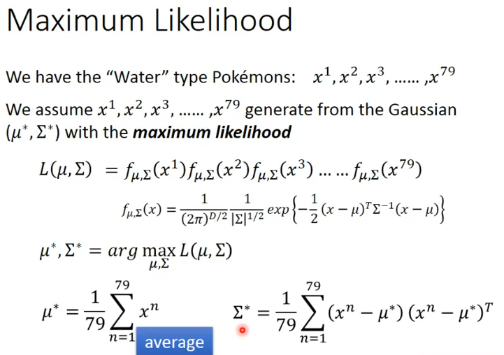
# Maximum Likelihood

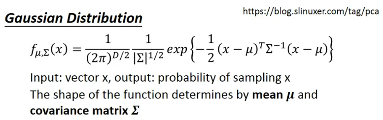
假設input是一個x,output是會隨著function帶入mean和covariance matrix後所得到的分佈也會有所不同
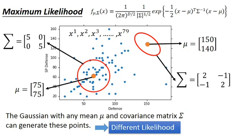
而為了要找到最大似然值，其實有一個最快的解法就是將function求導,就可以找到極大值
而對於正態分佈的模型，樣本的均值就是最大似然估計

# General Guide