# How to Build a SNARK that Is Out of This World :milky_way:

In the first section, we build up a very generic IPS. After carefully choosing the class of constraints, we find that the proof system practically writes itself. The structure of the statement to be proved determines the structure of the proof.

In more detail, we define the "base equations" that define a relation, see that each set of base equations defines not just a single relation, but a hierarchy of them. We note that using the reductions of knowledge framework of [[KP22](https://eprint.iacr.org/2022/009)] one strategy for a generic interactive protocol for any statement in the hierarchy consists of two stages: first the prover and verifier perform a series of reductions of knowledge to reduce verification to checking a statement at the bottom of the hierarchy, then use (potentially quite different) standard techniques to check this statement. Identifying these stages with the verifier and decider in [[BCMS20](https://eprint.iacr.org/2020/499), [BCLMS21](https://eprint.iacr.org/2020/1618)] we get an accumulation scheme for our protocol for free by applying the compiler of [[BCLMS21](https://eprint.iacr.org/2020/1618)].

In the second section, we describe a wide array of protocols as instantiations or optimizations of this generic protocol. (In particular, the IPS is not succinct but becomes succinct when the prover sends a commitment to their messages rather than the full message.)

The survey includes
- Recent "Out of This World" folding and accumulation schemes (Nova, HyperNova, Protostar)
- Recent work in folding and accumulation schemes with more terrestrial names (Sangria, Origami/Moon Moon, Halo2)
- Sum-Check arguments (Classical Sum-Check, Inner Product Arguments)
- Miscellaneous other protocols to demonstrate the flexibility of the framework (including Schnorr proofs, hinting at [[Mau09]](https://crypto.ethz.ch/publications/files/Maurer09.pdf)'s generalization)

In the third section I try to use this new framework to make qualitative comparisons between many of the protocols described in the second section. I offer an opinionated taxonomy of folding vs. accumulation (and their many variants). Finally I pose an open question using the language of the new framework.

## Build a generic SNARK
I'm going to introduce a class of indexed relations as generalizations of R1CS and we’re going to generalize it in two ways
- We’re going to swap out the constraint equations (like in [CCS](https://eprint.iacr.org/2023/552.pdf))
- We’re going to allow verifier input in the constraints (helpful for lookups, grand products, efficiency)

It's harder to genuinely simplify things than it is to just move the complexity around. Hopefully once we build up some definitions, all the recent work on folding and accumulation becomes easy, but that does mean we start with some tedious definitions.

An NP relation is a two-place predicate $\mathcal{R}(\cdot, \cdot)$ (usually defined on strings, because computer science) such that
- Given $(x,y)$, computing the truth value of $\mathcal{R}(x,y)$ can be done by a "verifier" in deterministic polynomial time.
- The length of $y$ is polynomially bounded by the length of $x$.

For every NP relation there is a language (i.e. a one-place predicate defined on strings) associated with $\mathcal{R}$, namely
$$ \mathcal{L(R)} = \{ x : (\exists y)[\mathcal{R}(x,y)] \ \}. $$
$\mathcal{L(R)}$ is a bona fide NP language, like from your CS classes or numberphile videos. The "$x$" that may or may not be in the language is called the *instance*. Any $y$ such that $\mathcal{R}(x,y)$ holds is called a *witness*.

Indexed relations extend the notion of an NP relation. An indexed relation is a triple consisting of an index, an instance, and a witness. They were introduced in [[CHM⁺19](https://eprint.iacr.org/2019/1047)] to formalize pre-processing SNARKs. The idea was that the index would encode the circuit, so you can formalize a pre-processing step as a procedure that depends only on the index. Then public inputs are part of the instance. For us it’s helpful because many of these folding schemes are defined as folding two relations that have the same structure, and we can formalize that notion as the relations having the same index.

Here's our prototypical SNARKable indexed relation, R1CS: The index consists of
- a ring $R$ with $R \cong \mathbb{F}^n$
- $\mathcal{A,B,C,P}:R \to R$, $\mathbb{F}$-linear functions, $\mathcal{P}$ a projection
- a pair of variables, $X, Z$
- a pair of expressions called constraint equations
$$\mathcal{P}(Z) = X \\ \mathcal{A}(Z)\circ\mathcal{B}(Z) = \mathcal{C}(Z).$$

The instance is a ring element $A \in R$, which is assigned to the variable $X$. A valid witness is a ring element $B \in R$ that when assigned to $Z$ makes the pair of expressions true.

In the definition of an NP relation, the instance and witness can be very general. There's no restriction other than the length. In contrast, the instance and witness for R1CS are very concrete. As we've presented it, it's also very simple (just a ring element) and the relation can be described using just algebraic terminology. (Again, moving complexity around rather than eliminating it. Now you need to know what a ring is. (But not really, by assumption that it is isomorphic to $\mathbb{F}^n$.))

### Build class of base equations
Our first step to generalization is to extend the class of constraint equations. We want to be able to build a SNARK for every relation in the class, so we can’t go too crazy with them.

For motivation, checking the validity of an assignment of $Z$ for R1CS frequently gets broken down into *lincheck* and *row-check*. (To my knowledge, this breakdown first appears in [[BCR⁺19]](https://eprint.iacr.org/2018/828.pdf) and [related talks](https://youtu.be/chURtuAgeWY?t=1393).) For vectors/ring elements $A,B,C$, a lincheck protocol verifies that
$$ \mathcal{A}(Z) = A \\ \mathcal{B}(Z) = B \\ \mathcal{C}(Z) = C $$
And a row-check protocol checks that the expression
$$ A \circ B -C =0 $$
holds as an expression over the ring. (For the usual case of vectors in $\mathbb{F}^n$, the multiplication $\circ$ is the hadamard product. When the ring is interpolating polynomials modulo a vanishing polynomial or vanishing ideal, this is also a point-wise multiplication.)

This is still a higher level of abstraction than polynomial IOPs and there's not necessarily a canonical way to turn it into a polynomial IOP. For example,
- Aurora [[BCR⁺19](https://eprint.iacr.org/2018/828.pdf)] and Marlin [[CHM⁺19](https://eprint.iacr.org/2019/1047)] reduce lincheck to univariate sum-check
- Spartan [[Set20](https://eprint.iacr.org/2019/550)] reduces lincheck to multivariate sum-check
- [[BCG20](https://eprint.iacr.org/2020/1426)] reduces lincheck to a “twisted scalar product” check

And the row-check is frequently glossed over as "standard techniques".

The fact that checking an R1CS witness can be reduced to linchecks and row-checks is an immediate corollary of the fact that the left hand side of the constraint equation
$$ \mathcal{A}(Z)\circ\mathcal{B}(Z)-\mathcal{C}(Z) = 0 $$
is representable with the following abstract syntax tree.

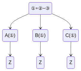[](https://mermaid-js.github.io/mermaid-live-editor/edit#pako:eNqrVkrOT0lVslIqLkksSXXJTEwvSszVLTOKyVMAgkcTFzzqmPFo4sJHHZMeTVykoKtrp-CoARTVhMhD2GDhqEcN3bg1OSFpckLVhFefM5I-ZyR9YBElHaXc1KLcxMwUoPurQUIxSiUZqbmpMUpWQGZKalpiaU5JjFJMXi1QaWJpSX5wZV6yklVJUWmqjlJpQQrCx0pWaYk5xUDR1JTMkvwiX0iYgIOmFgC7im6D)

So to generalize a proof system to other constraint equations, we represent the equations as abstract syntax trees. If we have an abstract syntax tree, we can check the input/output at each node with a sub-protocol. If we use a context free grammar, your [parse trees](https://en.wikipedia.org/wiki/Parse_tree) become ASTs, and the class of constraint equations generated has exactly the closure properties we want. (We can think of polynomials as the simplest class of functions closed under $\circ, +$ and containing the identity function and constant functions. Similarly, every set of linear functions on $R$ will define a class of "$\mu$-polynomials" which contain the identity and constant functions and are closed under $\circ,+$, and application of those linear functions.)

So the indexed relation R1CS generalizes immediately:
- Index is a set of $\mu$-polynomial equations
- Instance is an assignment of some of the variables
- A valid witness is a satisfying assignment of the remaining (free) variables

And we have a proof system for it! Neat!

As a note, the customizable constraint systems (CCS) of [[STW23](https://eprint.iacr.org/2023/552)] are a special case of $\mu$-polynomials and are also generated by a context-free grammar. They are a very well-chosen class of constraints, as it allows the linchecks to be batched; this is subtly implied by the differences between the grammar that generates $\mu$-polynomials and the grammar that generates CCS constraints. More research on connections between constraint generation and proof generation to come?

### Adding interaction
Image: a nested venn diagram where the outer layer is “relations” and the inner layer is “relations defined by a \mu-polynomial equation”
Question: is there an interesting layer between these two? Answer: Yes! (maybe)
Define a hierarchy of relations on each set of base equations

When we ask, "is $A$ in $\mathcal{L(R)}$?" we can't just say, "well, is $(A,W)$ in $\mathcal{R}$?" That question doesn't have a true/false answer, because it's not true or false, it's contingent on the value of $W$. For the purposes of interactive arguments, the prover will provide a satisfying value of $W$. To answer "is $A$ in this NP language" we can say, "well, is there an assignment $B \leftarrow W$ such that $(A,B)\in \mathcal{R}$ is a true statement?"

So this is how we generalize the indexed relations we've considered
- Index is still a set of $\mu$-polynomial equations
- Instance is a generalized assignment of some of the variables
- variables can be assigned a ring element (instantiated)
- or they can be quantified (though note the order of the quantifiers matters)
- Witness is still a satisfying assignment of the remaining (free) variables

Now borrowing from recursion theory, there's a way to categorize these relations in a hierarchy based on the structure of the sentences which define them.

A set of $\mu$-polynomial equations in $k$ variables defines a predicate on $R^k$. The predicate is essentially "does the equation hold when you plug in these $k$ values?" The predicate is said to be $\Sigma_0^{Q\mu}$ and $\Pi_0^{Q\mu}$, or simply "quantifier free" if they are just equations, with no quantifiers. For example, the predicate $\Phi$ defining R1CS,
$$ \Phi(X,Z) \equiv \begin{cases} \mathcal{P}(Z) = X \\ \mathcal{A}(Z) \circ \mathcal{B}(Z) = \mathcal{C}(Z) \end{cases}$$
has no quantifiers. Therefore we will also say that the relation R1CS is a $\Sigma_0^{Q\mu}$ and $\Pi_0^{Q\mu}$ relation. This may be a bit confusing, because we generally ask "does there exist a satisfying witness?" and shouldn't that be an existentially quantified statement? Is R1CS a $\Sigma_1^{Q\mu}$ relation?

Honestly, that is the approach I tried first. It is unpleasant to work with. Trust me that it is much easier to work with contingent statements involving free variables, and note that the index-instance pair (a set of $\mu$-polynomial equations and a generalized partial assignment of variables) defines a canonical indexed relation, where the witness is an assignment of the remaining variables.

The rest of the hierarchy is defined inductively. A predicate $\Phi$ is $\Sigma_{k+1}^{Q\mu}$ if
$$ \Phi(\vec X) \equiv (\exists \vec Y)\big[ \Psi(\vec X, \vec Y) \big] $$
for a $\Pi_k^{Q\mu}$ predicate $\Psi$. An indexed relation is $\Sigma_{k+1}^{Q\mu}$ if its defining predicate is $\Sigma_{k+1}^{Q\mu}$.

Dually, a predicate $\Phi$ is $\Pi_{k+1}^{Q\mu}$ if
$$ \Phi(\vec X, \vec y) \equiv (\forall \vec y)\big[ \Psi(\vec X, \vec y) \big] $$
for a $\Sigma_k^{Q\mu}$ predicate $\Psi$. An indexed relation is $\Pi_{k+1}^{Q\mu}$ if its defining predicate is $\Pi_{k+1}^{Q\mu}$.

### Reductions of Knowledge
So we've extended the set of relations under consideration, but our scheme for a proof of knowledge (write the predicate as an AST, provide a sub-proof at each node) says nothing about quantifiers! This isn't a huge issue, as we can use *reductions* of knowledge rather than full proofs (arguments).

First we'll cover (refresh on) reductions for languages/predicates. A reduction for a predicate is a way of converting one predicate $P$ to another predicate $Q$ in such a way that the truth value of $Q(x)$ can be used to determine $P(x)$. There are two often-used methods for how the solution to the second problem can be used. One is to use the decision procecure for $Q$ as a sub-routine for the decision procedure for $P$. Another method (the method we're interested in) is when a reduction is a function from instances to instances. So you might have a reduction function $f$ where $P(x) \iff Q(f(x))$. It's a pretty essential concept in theoretical computer science, so don't trust me for an exposition.

[[KP22](https://eprint.iacr.org/2022/009)] extend the notion to relations and specifically knowledge relations. So it's more like "the prover knows a witness for $P(x)$ iff they know a witness for $Q(f(x))$". (They did not invent the technique, but to my knowledge that was the first general formalization of it.)

The formalization of this (and the proper definitions of soundness, etc.) can be found in [[KP22](https://eprint.iacr.org/2022/009)]. The paper also proves that such reductions remain knowledge-sound when composed. This gives us a high-level strategy for proofs of knowledge for all of the relations in our hierarchy: first, compose reductions of knowledge to reduce to a $\Pi_0^{Q\mu}$ relation; then use the AST sub-proof method to prove the $\Pi_0^{Q\mu}$ statement.

With this concept, folding and accumulation schemes become easier to define.

### Accumulation Schemes & Folding Schemes

An atomic accumulation scheme is a reduction of knowledge from $R\times P$ to $P$. Here $P$ is a predicate rather than a relation, but we can think of this as a relation with null witness. It is also required that the reduction verifier runs more efficiently than the verifier for $P$, and that the verifier for $P$ (what they call the "decider" (because it decides a language)) is non-interactive, and doesn't get additional help from any kind of prover.

A split accumulation scheme is a reduction of knowledge $R \times Q$ to $Q$ (where $Q$ is a relation, specifically an instance-witness pair). It has the same efficiency requirements for the verifier, and the decider is still non-interactive. However the inclusion of a witness can assist in the decision.

Informally, a folding scheme is a reduction of knowledge specifically from $R \times R$ to $R$. It is most interesting when the verifier for the knowledge reduction is asymptotically more efficient than the verifer for $R$ itself.

### Simple Geometric Reduction

The prototypical knowledge reduction protocol is the sum-check protocol. (It's this protocol that [KP22] uses as an illustration.) Here is a simpler reduction for relations within our hierarchy. It is so simple that it is not necessarily sound.

| Simple Geometric Reduction |
| -------- |
| The prover, verifier, and decider agree on a field $\mathbb{F}$, a ring $R$ that is an $\mathbb{F}$ algebra, a set of $\mathbb{F}$-linear functions $\mathcal{F}$ from $R$ to $R$, base equations $\Phi$, and instance $A$. <br> 1. If $\vec A \in \mathcal{L(R}_1)$ if and only if $$ (\forall \vec y)\big[ \Phi(\vec A, \vec y) \big]$$ <br>the verifier sends a random assignment $$ \vec c \leftarrow \vec y $$ where $\vec c$ is drawn uniformly from $\mathbb{F}$. <br> 2. If $\vec A \in \mathcal{L(R}_1)$ if and only if $$ (\exists \vec W)\big[ \Phi(\vec A, \vec W) \big]$$ <br>the prover sends a satisfying assignment of variables $$\vec B \leftarrow \vec W$$ 3. The verifier queries the decider and accepts if $(\vec A, \vec c) \in \mathcal{R}_2$ or $(\vec A, \vec B) \in \mathcal{R}_2$ |

Special sound protocols with algebraic verifiers and Pi_0 accumulator checks are in one-to-one correspondence with these proofs

[[AFK22](https://eprint.iacr.org/2021/1377)]

Using the generic compiler, we get an accumulation scheme where the verifier checks the reductions of knowledge and the decider checks the Pi_0 statement

## Generalizations, Instantiations, and Optimizations

Let $\phi(Z)$ be a degree $d$ homogenous polynomial of the form $\alpha(Z) - \delta(Z)$ for $\alpha, \delta$ homogenous of degree $d$. Then the unfolding extension/relaxation is the predicate
$$ (\forall y)(\exists Z)\big[ \phi_{relaxed}(W_1, W_2, T, y, Z) \big] $$
$$ \phi_{relaxed}(Z,T) = \begin{cases}
Z = W_1 + y W_2 \\
\mathcal{P}(Z) = X_1 +y X_2 \\
\phi(Z) = \phi(W_1) + y^d \phi(W_2) - \epsilon(T)
\end{cases}$$

**Nova**
The homogenization of the R1CS equations (with homogenizing variable $u$) is
$$ \Phi(X,Z) \equiv \begin{cases} u \mathcal{P}(Z) -u X = 0 \\ \mathcal{A}(Z) \circ \mathcal{B}(Z) - u \mathcal{C}(Z) = 0 \end{cases}$$

**Inner Product Argument**
The field $\mathbb{F}$ embeds in the ring $R$ by sending each $a \in \mathbb{F}$ to the vector where every entry is $a$. Then for any $X \in R$, the scalar product $aX$ is equal to the hadamard product $embed(a) \circ X$ (so we'll just identify field elements with their embedding in the ring).

Letting $\mathcal{s}$ be the matrix of all ones, the inner product relation $\langle A, B \rangle = c$ can be written as a $mu$-polynomial expression $\mathcal{S}(A \circ B) = c$.

**Sum-Check Argument**
This clearly generalizes to $\mathcal{S}(f(Z)) = c$ for any polynomial function $f$ of ring elements $Z$.

**Schnorr's ZKPoK of a Discrete Logarithm**
So far we have glanced over the fact that the accumulation prover is not sending witnesses in the clear, but rather their image under a homomorphic commitments. A full treatment of the necessary properties of the commitment scheme in a related class of "foldable" relations (with proofs) can be found in [[BCS21](https://eprint.iacr.org/2021/333)] , and our treatment of Schnorr's ZKPoK is only meant to hint at how the distinction between witness and commitment can be handled.

The discrete log relation is an indexed relation where the index comprises a cyclic group and choice of generator $g$, the instance is an element of the group $h$, and the witness is an integer $x$ such that $h = g^x$ in the group (but you knew this already). [Schnorr's protocol for proof of knowledge](https://crypto.stanford.edu/cs355/19sp/lec5.pdf) for this relation, a standard first example of proofs of knowledge, can be understood in the context of folding.

The prover's first move is to generate a uniformly random instance with the same index $u=g^r$ (by choice of a random witness $r$). The prover and verifier then perform the standard folding protocol to reduce knowledge of a witness for the original instance/witness pair $(h, x)$ and the randomly sampled instance/witness pair $(u, r)$ to a third pair $(u\cdot h^c, z)$ where the prover can send the witness $z$ in the clear. There are no "cross-terms" because the relation between $x$ and $h$ is "linear" in a sense.

**Sangria**
Note that the implied arithmetization from the PlonK protocol is not immediately $\Pi_0$. An important insight of [[Moh23](https://github.com/geometryresearch/technical_notes/blob/main/sangria_folding_plonk.pdf)] is that this does not matter, as a folded wiring assignment will also pass the permutation check.

There is some ambiguity around what "plonk-ish arithmetization" means, but the usual meaning is slightly different than what we mean by "implied arithmetization". Roughly, an interactive protocol has an algebraic verifier if the final verification check is checking a closed [i.e. having no un-assigned variables], quantifier-free arithmetic expression in a certain ring. "Forgetting" the variable assignments, we get the base equations of the relation, which are quantifier-free predicates, but have free variables. Each message from the verifier binding a variable to a challenge can be thought of as placing a universal quantifer on that variable. Each message from the prover binding a response to a variable can be thought of as placing an existential quantifier on that variable.

Therefore, because the permutation argument of PlonK has the verifier sending a challenge and the prover sending an accumulation polynomial, the implied arithmetization, in plain English, is something like "for all challenges $\beta, \gamma$ there exists an accumulator polynomial $Z(X)$ such that [constraints hold]". Thus the implied constraints are at least $\Pi_2$ and relate the wiring assignments, challenges, and accumulator.

However, this is equivalent to a $\Pi_0$ $\mu$-polynomial constraint. This is perhaps obvious for a single wiring/witness polynomial (a simplifying assumption made in [[BC23](https://eprint.iacr.org/2023/620.pdf)]). To extend the proof to permutations "across wires" as in the original PlonK paper, it suffices to check permutations pairwise between wires.

Thus the wiring assignment for PlonK is $\Pi_0$, and therefore its relaxed version is foldable, but interestingly the copy constraints on a folded witness can be checked with the more efficient 3-move permutation argument.

<u>**Non-tensor &Pi;_2k relations, k &gt; 0**</u>
Many interactive protocols have $\Theta(\log n)$ moves where the $\log n$ factor comes from a recursive halving of the size of the instance. [BCS21] and [[KP22](https://eprint.iacr.org/2022/009)] attribute this to a "tensor structure". Some protocols use multiple rounds that aren't "halving". A prominent example is the grand product sub-argument used in PlonK, plookup, Halo2lookup, and others. As mentioned in the section on Sangria, PlonK's $\Pi_2$ grand product constraints are equivalent to a $\Pi_0$ set of copy constraints. The grand product as used in Halo2lookup is not.

**Origami/Moon Moon/Halo2**
[Halo2lookup](https://zcash.github.io/halo2/design/proving-system/lookup.html) is a simple lookup protocol for use with plonk-ish systems. The prover re-orders a column of (alleged) lookup values from the circuit and a publicly known lookup table in column form. They then show that each alleged lookup value is equal to either the entry in the same position in the re-ordered table, or equal to a value in the alleged lookup column already constrained to be in the table. These constraints are not difficult to prove as part of a Sangria folding scheme, as they consist of pointwise operations and a shift.

The difficult part to fold is the grand product argument, where the re-ordering may scatter different entries of the lookup vector and table so they no longer line up as pointwise constrainable.

Solution? Run the interactive reduction (assigning variables) until you get to the $\Pi_0$ constraints (formerly quantified variables are now assigned). Fold the $\Pi_0$ constraints and assignments.

**ProtoStar**
[BC23] takes the same idea, which they identify as originating in [BCLMS21].

They also swap out the grand product-based lookup argument for one based on logarithmic derivatives. And apply a trick based on HyperNova's to reduce the need for cross-terms.

**ProtoGalaxy**
Is very recent work. Haven't looked at it yet. I cannot keep up with all this.

**HyperNova**
[[SWT23](https://eprint.iacr.org/2023/552.pdf)] introduced the customizable constraint system (CCS). It generalizes R1CS in that it's a polynomial function of a few "intermediate" values that specifically are linear transformations of the instance/witness vector. CCS constraints are still $\Pi_0$. Because CCS constraints are higher degree than R1CS, the standard unfolding/folding method introduces more cross-terms. (This is also an issue with Sangria.) HyperNova has a clever solution to get around this.

I wrote a good page or so that I decided to scrap bc the idea is simpler (more genius) than I initially realized. Recall that R1CS is proven with "standard methods" for the row-check and a more novel (sometimes) lincheck protocol. One standard method is to run the sum-check protocol on $\tilde{eq}(\tau,x)\cdot f(x)$ to see if it's the zero polynomial. Also recall that sum-check is less of a decision protocol and more a reduction protocol (reducing to evaluation of the polynomial at a random point). If $f(x)$ is a degree $d$ polynomial function of polynomials $\{f_1, \ldots f_t \}$ of degree $n$, evaluation of this composite takes $O(\log n + d)$ *field* operations given the evaluations of $\{f_1, \ldots f_t \}$. (In the case of CCS, these polynomials are the interpolations of $M_i\cdot Z$.) So the verifier can check a folding/accumulation as "correct, contingent on the claimed value of $\widetilde{M_i\cdot Z}(r_a)$ being correct." It's the oldest trick in the accumulation book.

So the multi-folding scheme of HyperNova is (as noted by authors of both papers) very similar to split accumulation schemes. The prover and verifier perform a very accumulation-like reduction to reduce a *single instance* of CCS to "linearized CCS" and then perform a more folding-like reduction to reduce two linearized CCS instances to one.

That is (in my opinion) the gist of how HyperNova works, but the actual protocol as described in the paper is more of an optimization. A more thorough exploration of how degree-reducing reductions can be interleaved with folding reductions is warranted, but a starting place is section 3.5 of ProtoStar.

## Analysis

The papers defining folding and accumulation schemes define them (in the academic tradition) with bit strings as the primitive notion. The Nova paper, in introducing folding schemes focused on *non-trivial* folding schemes where "non-trivial" specifically meant having lower communication complexity than sending a proof of one of the statements. The accumulation schemes duology similarly requires the accumulation verifier to receive only a short instance rather than a potentially long witness.

The motivation in my presentation is to constrain both the communication and more importantly the allowed reduction work to better capture the structure of existing folding/accumulation schemes rather than just size.

For example, it is known that IVC and PCD can be realized from a SNARK with fully sublinear verification. [KST22] specifically rules this out as a non-example of a non-trivial folding scheme. Sangria was quite exciting when it came out because it allowed plonk-ish arithmetizations to be folded. However it is known that R1CS is NP-complete, so a folding scheme for plonk-ish already existed: convert the plonkish instance to an R1CS instance and fold with Nova.

The accumulation scheme duology is all about finding a weaker condition than full sublinearity that suffices for PCD. I'm taking the opposite approach, namely, "here's a stricter notion of reduction that still suffices to express folding/accumulation."

This document is advocating for a perspective where we consider SNARKs where the only reduction step is a randomized variable assignment, and this forms a sort of [many-one reduction](https://en.wikipedia.org/wiki/Many-one_reduction) to evaluating expressions in a ring. A linear combination of these expressions can be evaluated to probabilistically check all of them. Therefore these expressions form an accumulator for these relations. The reduction to quantifier-free expressions (normally just called "expressions") corresponds to the accumulation prover/verifier or folding prover/verifier interaction and results in a full assignment of all variables. Checking that the assignment satisfies the proper polynomial constraint/expression done by the "decider".

So in this light, very roughly, the accumulation line of work says that you can fold proofs together after creating them whereas the folding line of work says that you can accumulate statements to prove before actually checking them. Proofs are "points" which are accepted only if some polynomials vanish at that point. Statements are (generalized) polynomial expressions but can be considered points in a more complicated ring. This largely makes the difference a matter of perspective.

## Open Question?
Does there exist a folding scheme for a relation whose defining predicate is not quantifier-free [for some choice of ring]?

Example: as noted, wiring assignments for vanilla plonk are $\Pi_0$ (so not defined by any verifier challenges). The halo2 lookup relation is $\Pi_2$, requiring a verifier challenge to construct the grand product polynomial. Current folding schemes for this relation simulate the verifier's challenge with a random oracle. Is there a lookup argument that works on folded wire assignments without creating the grand product?