## Week 1: Mastering Clustering and Unsupervised Machine Learning

### 📅 DAY 1: Introduction to Unsupervised Learning and Clustering

#### a. **Unsupervised Learning: Discovering Hidden Patterns**
Unsupervised learning is a type of machine learning that looks for previously undetected patterns in a dataset with no pre-existing labels and with a minimum of human supervision. Unlike supervised learning, there are no predefined target variables. The goal is to identify patterns, groupings, or structures within the data.

🔍 **Learn More:**
Get started with this comprehensive overview on [**unsupervised learning**](https://www.altexsoft.com/blog/unsupervised-machine-learning/).

#### b. **Clustering: Grouping Data Intelligently**
Clustering is a fundamental unsupervised learning technique used to group similar data points together. It aims to divide the data into clusters, where points in the same cluster are more similar to each other than to those in other clusters.

🔍 **Discover Clustering:**
Dive into clustering basics with [**this guide**](https://towardsdatascience.com/overview-of-clustering-algorithms-27e979e3724d).

---

### 📅 DAY 2: K-Means Clustering

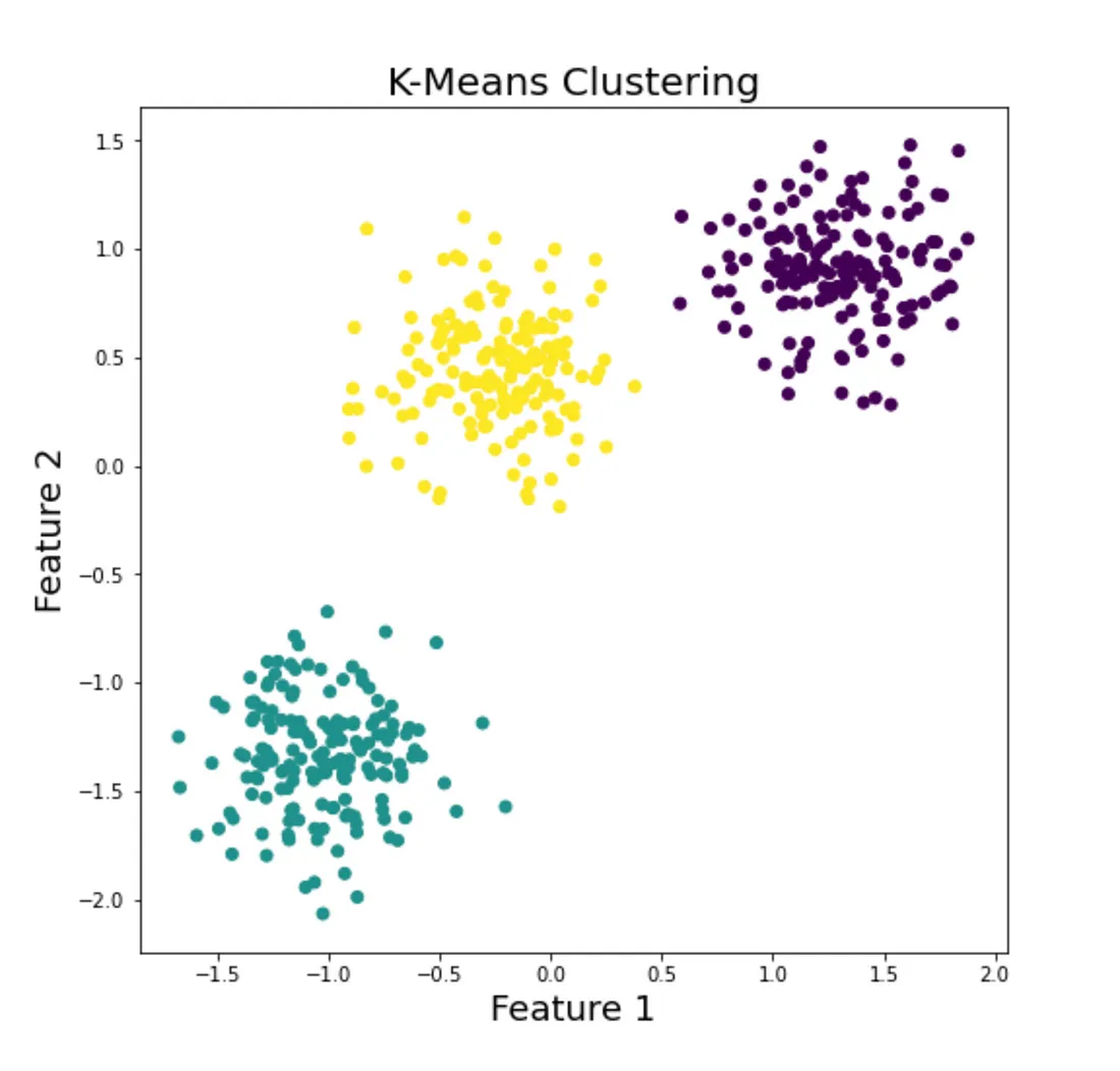
#### a. **Understanding K-Means Clustering**
K-Means is one of the simplest and most popular clustering algorithms. It partitions the data into K clusters, where each data point belongs to the cluster with the nearest mean. This iterative process aims to minimize the variance within each cluster.

🧠 **How It Works:**
1. Initialize K centroids randomly.
2. Assign each data point to the nearest centroid.
3. Update centroids by calculating the mean of the assigned points.
4. Repeat until convergence (centroids no longer change).

🔍 **Explore More:**
Learn about K-Means in detail [**here**](https://www.analyticsvidhya.com/blog/2019/08/comprehensive-guide-k-means-clustering/).

#### b. **Hands-On with K-Means**
Get hands-on experience by implementing K-Means clustering in Python.

🔍 **Follow Along with Code:**
Check out this step-by-step tutorial on K-Means implementation [**here**](https://realpython.com/k-means-clustering-python/).

---

### 📅 DAY 3: Hierarchical Clustering

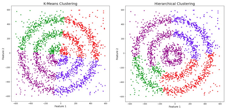
#### a. **Hierarchical Clustering: Building Nested Clusters**
Hierarchical clustering builds a hierarchy of clusters. It can be divided into Agglomerative (bottom-up approach) and Divisive (top-down approach) clustering.

🧠 **How It Works:**
- **Agglomerative:** Start with each data point as a single cluster and merge the closest pairs iteratively until all points are in a single cluster.
- **Divisive:** Start with one cluster containing all data points and recursively split it into smaller clusters.

🔍 **Deep Dive:**
Understand hierarchical clustering with this [**guide**](https://www.javatpoint.com/hierarchical-clustering-in-machine-learning).

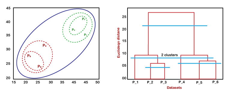
#### b. **Visualizing Dendrograms**
Dendrograms are tree-like diagrams that illustrate the arrangement of clusters produced by hierarchical clustering. They help to visualize the process and results of hierarchical clustering.


---

### 📅 DAY 4: Density-Based Clustering (DBSCAN)

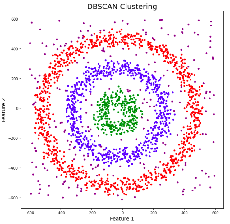
#### a. **DBSCAN: Clustering Based on Density**
Density-Based Spatial Clustering of Applications with Noise (DBSCAN) is a clustering algorithm that groups together points that are closely packed and marks points that are far away as outliers. It is particularly effective for datasets with noise and clusters of different shapes and sizes.

🧠 **How It Works:**
1. Select a point and find all points within a specified distance (epsilon).
2. If there are enough points (minimum samples), form a cluster.
3. Expand the cluster by repeating the process for each point in the cluster.
4. Mark points that don't belong to any cluster as noise.

🔍 **Learn More:**
Understand DBSCAN and its code in detail [**here**](https://scikit-learn.org/stable/modules/clustering.html#dbscan).

#### b. **Implementing DBSCAN**
Get practical experience by implementing DBSCAN in Python.

🔍**Take a look at the documentation:**
You can go through the sklearn documentation for a better insight of DBSCAN.
https://scikit-learn.org/stable/auto_examples/cluster/plot_dbscan.html#sphx-glr-auto-examples-cluster-plot-dbscan-py

https://scikit-learn.org/stable/modules/generated/sklearn.cluster.DBSCAN.html

---

### 📅 DAY 5: Evaluation Metrics for Clustering

Clustering is only useful if we can evaluate the quality of the clusters it produces. This day will focus on understanding and using various metrics to assess clustering performance. These metrics help us determine how well our clustering algorithms are grouping similar data points and separating dissimilar ones.

#### a. **Silhouette Score**

**Definition:**
The silhouette score measures how similar an object is to its own cluster compared to other clusters. It ranges from -1 to 1, where a high value indicates that the object is well matched to its own cluster and poorly matched to neighboring clusters.

**How It Works:**
- For each data point:
1. Calculate the average distance to all other points in the same cluster (a).
2. Calculate the average distance to all points in the nearest cluster (b).
3. The silhouette score for a point is given by:

$$
s = \frac{b - a}{\max(a, b)}
$$

- The overall silhouette score is the average of individual silhouette scores.

#### b. **Davies-Bouldin Index**

**Definition:**
The Davies-Bouldin Index (DBI) measures the average similarity ratio of each cluster with the cluster that is most similar to it. Lower DBI values indicate better clustering as they represent smaller within-cluster distances relative to between-cluster distances.

**How It Works:**
- For each cluster:
1. Compute the average distance between each point in the cluster and the centroid of the cluster (within-cluster scatter).
2. Compute the distance between the centroids of the current cluster and all other clusters (between-cluster separation).
3. Calculate the DBI for each cluster and take the average.
4. The DBI is given by:
$$
\text{DBI} = \frac{1}{N} \sum_{i=1}^{N} \max_{j \neq i} \left( \frac{s_i + s_j}{d_{ij}} \right)
$$
where s_i and s_j are the average distances within clusters \(i\) and \(j\), and \(d_{ij}\) is the distance between the centroids of clusters \(i\) and \(j\).

#### c. **Adjusted Rand Index (ARI)**

**Definition:**
The Adjusted Rand Index (ARI) measures the similarity between two clusterings by considering all pairs of samples and counting pairs that are assigned in the same or different clusters in the predicted and true clusterings. It adjusts for chance grouping.

**How It Works:**
- Compute the Rand Index (RI):
1. Count pairs of points that are in the same or different clusters in both true and predicted clusters.
2. The RI is the ratio of the number of correctly assigned pairs to the total number of pairs.
- Adjust the RI to account for chance clustering, resulting in ARI.

**Formula:**
$$
\text{ARI} = \frac{\text{RI} - \text{Expected\_RI}}{\max(\text{RI}) - \text{Expected\_RI}}
$$

#### d. **Practical Guide to Evaluating Clusters**

1. **Silhouette Analysis**:
- **When to Use:** To determine the optimal number of clusters and understand cluster cohesion and separation.
- **Practical Example:** Implement silhouette analysis using Python’s scikit-learn library to evaluate K-means clustering results.

2. **Davies-Bouldin Index**:
- **When to Use:** To assess the quality of clustering where the clusters are of different shapes and sizes.
- **Practical Example:** Use the Davies-Bouldin Index to compare different clustering algorithms on a given dataset.

3. **Adjusted Rand Index**:
- **When to Use:** To compare the clustering results with ground truth labels.
- **Practical Example:** Compute the ARI to evaluate the clustering performance on a labeled dataset, such as customer segments with predefined categories.

🔍 **Explore Metrics in Practice:**
Explore the given metrices and its computation [**here**](https://www.geeksforgeeks.org/clustering-metrics/).

#### e. **Visualizing Clustering Results**

Visualization is a powerful tool for interpreting and presenting clustering results. Common visualization techniques include:
- **Scatter plots**: Useful for low-dimensional data, showing cluster assignments and centroids.
- **Heatmaps**: Visualize distance matrices or similarity matrices.
- **Dendrograms**: Illustrate the hierarchical clustering process.

---

### 📅 DAY 6: Dimensionality Reduction Techniques

Dimensionality reduction is crucial in unsupervised learning as it helps in simplifying models, reducing computation time, and mitigating the curse of dimensionality. This day will focus on understanding and applying different techniques for reducing the number of features in a dataset while preserving as much information as possible.

#### a. **Principal Component Analysis (PCA)**(**Already discussed**)

#### b. **t-Distributed Stochastic Neighbor Embedding (t-SNE)**

**Definition:**
t-SNE is a nonlinear technique for dimensionality reduction that is particularly well suited for visualizing high-dimensional datasets. It converts similarities between data points to joint probabilities and tries to minimize the Kullback-Leibler divergence between the joint probabilities of the low-dimensional embedding and the high-dimensional data.

**How It Works:**
- Compute pairwise similarities in the high-dimensional space.
- Define a probability distribution over pairs of high-dimensional objects.
- Define a similar distribution over the points in the low-dimensional space.
- Minimize the Kullback-Leibler divergence between these two distributions using gradient descent.

🔍 **Learn More:**
Understand the intricacies of t-SNE and its implementation [**here**](https://distill.pub/2016/misread-tsne/).

#### c. **Linear Discriminant Analysis (LDA)**

**Definition:**
LDA is a linear technique used for both classification and dimensionality reduction. It aims to find a linear combination of features that best separates two or more classes of objects or events. LDA is particularly useful when the data exhibits clear class separations.

**How It Works:**
- Compute the mean vectors for each class.
- Compute the scatter matrices (within-class scatter and between-class scatter).
- Compute the eigenvalues and eigenvectors for the scatter matrices.
- Select the top k eigenvectors to form a new matrix.
- Transform the original data using this matrix to get the reduced dataset.

🔍 **Learn More:**
Dive deeper into LDA and its application [**here**](https://sebastianraschka.com/Articles/2014_python_lda.html).

#### d. **Uniform Manifold Approximation and Projection (UMAP)**

**Definition:**
UMAP is a nonlinear dimensionality reduction technique that is based on manifold learning and is particularly effective for visualizing clusters in high-dimensional data. It constructs a high-dimensional graph of the data and then optimizes a low-dimensional graph to be as structurally similar as possible.

**How It Works:**
- Construct a high-dimensional graph representation of the data.
- Optimize a low-dimensional graph to preserve the topological structure.
- Use stochastic gradient descent to minimize the cross-entropy between the high-dimensional and low-dimensional representations.

🔍 **Learn More:**
Learn about UMAP and its effectiveness in data visualization [**here**](https://umap-learn.readthedocs.io/en/latest/).

#### e. **Practical Guide to Dimensionality Reduction**

1. **Principal Component Analysis (PCA)**:
- **When to Use:** When you need to reduce dimensions linearly and want to preserve variance.
- **Practical Example:** Use PCA to reduce the dimensions of a dataset before clustering.

2. **t-Distributed Stochastic Neighbor Embedding (t-SNE)**:
- **When to Use:** When you need to visualize high-dimensional data in 2 or 3 dimensions.
- **Practical Example:** Apply t-SNE to visualize customer segments in an e-commerce dataset.

3. **Linear Discriminant Analysis (LDA)**:
- **When to Use:** When you need to perform dimensionality reduction for classification tasks.
- **Practical Example:** Use LDA to reduce the number of features in a labeled dataset before applying a classifier.

4. **Uniform Manifold Approximation and Projection (UMAP)**:
- **When to Use:** When you need a fast and scalable way to visualize high-dimensional data.
- **Practical Example:** Employ UMAP to visualize clusters in genetic data.

🔍 **Explore Techniques in Practice:**
Learn how to apply these dimensionality reduction techniques using Python and real datasets in this [**comprehensive guide**](https://towardsdatascience.com/dimensionality-reduction-for-visualizing-machine-learning-datasets-430c85105a8d).

---

By the end of Day 6, you will have a thorough understanding of various dimensionality reduction techniques, how to implement them, and when to apply each method effectively. This knowledge will be crucial for handling high-dimensional data in unsupervised learning tasks. 🚀

---

### 📅 DAY 7: Practical Applications and Project Work

#### a. **Applying Clustering to Real-World Data**
Put your knowledge into practice by applying clustering algorithms to real-world datasets. This will solidify your understanding and help you tackle real-life problems.

🔍 **Try It Out:**
Explore practical clustering applications on [**kaggle**](https://www.kaggle.com/datasets).

#### b. **Project: Customer Segmentation**
Work on a project to segment customers based on their purchasing behavior. This project will help you understand how clustering can be used for market segmentation, personalized marketing, and more.

🔍 **Follow Along with Project:**
Check out this customer segmentation project [**here**](https://www.kaggle.com/code/kushal1996/customer-segmentation/notebook).

---

By following this roadmap, you'll gain a strong foundation in clustering and unsupervised learning, empowering you to uncover hidden patterns and insights in your data. Happy clustering! 🚀