# 人工智慧期末考

---

# Chapter 19 - Learning from examples

Learning: make predictions after observating about the world

why agent need to learn
- no all possible situations were considered
- no all information about changes over time
- human have no idea how to program

---

## Supervised learning
given a training set $N$ = $(x_1, y_1), (x_2, y_2), ..., (x_N, y_N)$

假設真實世界中有一函數 $y = f(x)$
學習的目的就是要找出近似函數 $h \Rightarrow y \approx h(x)$

**The function $h$ is a hypothesis. Learning is a search through the space of possible hypotheses for one that will perform well, even on new examples beyond the training set.**

:::info
- Sometimes the function $f$ is stochastic, what we have to learn is a conditional probability distribution, $P(Y | x)$
:::

- $y \in$ finite set (boolean, binary) $\Rightarrow$ classification
- $y$ is a number $\Rightarrow$ regression

:::info
- Ockham’s razor (簡約法則)
- 同一個問題有許多種理論，每一種都能作出同樣準確的預言，那麼應該挑選其中使用假定最少的
- 儘管越複雜的方法通常能做出越好的預言，但是在不考慮預言能力（即結果大致相同）的情況下，假設越少越好
- prefer the simplest hypothesis
:::

- tradeoff
- complex hypotheses $\Rightarrow$ fit training data well
- simpler hypotheses $\Rightarrow$ may generalize better

- Supervised learning can be done by choosing the hypothesis h* that is most probable given the data:
- $h^* = argmax_{h \in H} P(h | data)$
- $h^* = argmax_{h \in H} P(data | h) * P(h)$
- By Bayes's rule

## Decision tree
A decision tree represents a function that inputs a vector of attribute values and returns a 『decision』

A decision tree reaches its decision by performing a sequence of tests


- An example for a Boolean decision tree consists of an (x, y) pair, where
- x is a vector of values for the input attributes
- y is a single Boolean output value

### Strategy of decision tree
- The algorithm adopts a greedy divide-and-conquer strategy:
- Always test the most important attribute first
- The $\it{IMPORTANCE}$ function
- Most important attribute, means the one that makes the most difference to the classification of an example
- Decision tree will be shallow
- Algorithm:
|  |
| -------- |

- Choosing the attribute tests
- Entropy: The entropy of a random variable V with values $v_k$, each with probability $P(v_k)$, is defined as
- $H(V) = \Sigma_k P(v_k)log_2\frac{1}{P(v_k)}$
- $H(V) = -\Sigma_k P(v_k)log_2{P(v_k)}$

- The entropy of a Boolean random variable that is true with probability q
- $B(q) = -(q)log(q) -(1-q)log(1-q)$

- If a training set contains p positive examples and n negative examples, then the entropy of the goal attribute on the whole set is
- $H(Goal) = B\lceil\frac{p}{p+n}\rceil$

- Remainder:
- An attribute A with d distinct values divides the training set $E$ into subsets $E_1$, ..., $E_d$
- Each subset $E_k$ has $p_k$ positive examples and $n_k$ negative examples
- If we go along that branch, we will need an additional $B(p_k/(p_k + n_k))$ bits of information to answer the question
- A randomly chosen example from the training set has the kth value for the attribute with probability $(p_k + n_k)/(p + n)$, so the expected entropy remaining after testing attribute A is
- $Remainder(A) = \Sigma^d_{k=1} \frac{p_k + n_k}{p + n} B(\frac{p_k}{p_k + n_k})$

- $\star$$\star$ Information Gain
- $Gain(A) = B(\frac{p}{p + n}) - Remainder(A)$
- This is the $\it{IMPORTANCE}$ function we need to implement

### Overfitting
- 訓練準確度很高，但遇到不在訓練資料內的測資時，準確度異常降低
- 即 model 不具一般性
- **Decision tree pruning** combats overfitting
- 合併末端分支 (leaf node)
- p: positive smaples
- n: negative smaples
- if 移除末端分支 $\Rightarrow$ 仍為 $\frac{p}{p + n}$
- Significant test (顯著性分析)
- 判斷跟背景樣態是否有顯著差別
- $\hat{p_k}, \hat{n_k}$: 背景值預估上的數量
- $p_k, n_k$: 實際上的值
- 其中，$\hat{p_k} = p \times \frac{p_k + n_k}{p + n}$、$\hat{n_k} = n \times \frac{p_k + n_k}{p + n}$
- $\Delta = \Sigma^d_{k=1} \frac{(p_k - \hat{p_k})^2}{\hat{p_k}} + \frac{(n_k - \hat{n_k})^2}{\hat{n_k}}$
- Early stopping
- Tree 長到一定程度便提前結束
- 沒有好的 attribute 便停止

### Broadening the applicability of decision tree
- Missing data
- Multivalued attributes
- Continuous and integer-valued input attributes
- Continuous-valued output attributes
- Use regression tree

## Evaluating and choosing the best hypothesis
- Independent and identically distributed (i.i.d.)
- Each example data point $E_j$ whose observed value $e_j = (x_j, y_j)$ and each example has an identical prior probability distribution
- $P(E_j | E_{j-1}, E_{j-2}, ...) = P(E_j)$
- $P(E_j) = P(E_{j-1}) = P(E_{j-2})$

- K-fold cross validation
- 將資料分成 k 個相等大小的 folds
- 接著執行 k 次訓練，每次訓練把其中一個 fold 當作 test set，剩下 k-1 個 folds 當作 training set
- 綜合評估這 k 次的 test score 會比單次評估的效果來得好

:::info
- When k = n, is calles LOOCV (leave-one-out cross validation)
:::

- Model selection
- 在 complexity 與 goodness of fit 之間權衡
- 決定使用哪種模型可以在 hypothesis space 不複雜的情況，同時達到較好的 fitting
- Finding the best hypothesis 可分為兩步驟
- Model selection: defines the hypothesis space
- Optimization: finds the best hypothesis within that space

- Loss function
- The loss function $L(x, y, \hat{y})$ is defined as the amount of utility lost by predicting $h(x) = \hat{y}$ when the correct answer is $f(x) = y$
- $L(x, y, \hat{y})$ = Utility(using y given x) - Utility(using $\hat{y}$ given x)
- L1 loss
- $L_1(y,\hat{y}) = |y-\hat{y}|$
- L2 loss
- $L_2(y,\hat{y}) = (y-\hat{y})^2$
- 0/1 loss
- $L_{0/1}(y,\hat{y})=0$ if $y=\hat{y}$ else 1
- Use $L_{0/1}$ loss for discrete-valued output
- Generalization loss --> 理想
- $GenLoss_L(h) = \Sigma_{(x,y)\in\epsilon}$ L(y,h(x)) P(x,y)
- The best hypothesis, $h^* = argmin_{h\in H} GenLoss_L(h)$
- Empirical loss --> 實際
- $EmpLoss_{L,E}(h) = \frac{1}{N} \Sigma_{x,y\in E} L(y,h(x))$
- $\hat{h^*} = argmin_{h\in H} EmpLoss_{L,E}(h)$

- Regularization
- Search for a hypothesis that directly minimizes the weighted sum of empirical loss and the complexity of the hypothesis
- $Cost(h) = EmpLoss(h) + \lambda Complexity(h)$
- $\hat{h^*} = argmin_{h\in H} Cost(h)$

## Regression and classification with linear models
- Univariated linear regression
- $h_w(x) = w_1x + w_0$
- $Loss(h_w) = \Sigma^N_{j=1} (y_i-(w_1x_j+w_0))^2$
- Find $w^* = argmin_w Loss(h_w)$
- $Loss(h_w)$ is minimized when its partial derivatives with respect to $w_0$ and $w_1$ are 0
- Every linear regression problem with $L_2$ loss function, the loss function is convex, and implies there are no local minima
- $w_i \leftarrow w_i - \alpha\frac{\partial}{\partial w_i} Loss(w)$
- $\alpha$ is called step size or learning rate
- gradient descent
- Batch gradient descent (BGD)
- slow and cost high
- Stohastic gradient descent (SGD)

- Multivariate linear regression
- Each example $x_j$ is an n-element vector
- $h_{sw}(X_j) = w_0 + \Sigma_i w_ix_{j,i}$
- $h_{sw}(X_j) = W \cdot X_j = W^T \cdot X_j = \Sigma_i w_ix_{j,i}$
- The best vector of weights, $w^*$
- $w^* = argmin_w \Sigma_j L_2(y_i,w\cdot x_j)$
- It is common to use regularization on multivariate linear regression to avoid overfitting
- $Complexity(h_w) = L_q(w) = \Sigma_i {|w_i|}^q$
- q = 1, $L_1$ regularization (absolute values)
- sparse model
- q = 2, $L_2$ regularization (squares)

- Logistic regression
- $h_w(X) = Logistic(W\cdot X) = \frac{1}{1 + e^{-W\cdot X}}$
- No easy closed-form solution to find the optimal value of w
- Use gradient descent
- Hypotheses no longer output just 0 or 1
- Use $L_2$ loss function

- Nonparametric model
- Would not be characterized by a bounded set of parameters
- Also called instance-based learning or memory-based learning
- Nearest neighbor (NN)
- $NN(k,x_q)$
- Cross-validation can be used to select the best value of k
- Minkowski distance ($L_p norm$)
- $L^p(X_j,X_q) = {(\Sigma_i {|x_{j,i} - x_{q,i}|}^p)}^{\frac{1}{p}}$
- Normalization $\frac{(x_{j,i}-\mu_i)}{\sigma_i}$
- Curse of dimensionality
- 維度越高，資料離越遠
- 利用 domain knowledge 降維
- K-d tree
- Locality-sensitive hashing (LSH)

## Support vector machines (SVM)
- Construct a maximum margin separator
- Create a linear separating hyperplane
- Kernel trick
- Nonparametric model
- The separator is defined as the set of points {x : w $\cdot$ x + b=0}
- Find the parameters that maximize the margin
- optimal solution
- $argmax_{\alpha} \Sigma_j \alpha_j-\frac{1}{2} \Sigma_{j,k} \alpha_j \alpha_k y_j y_k (X_j \cdot X_k)$
- where $\alpha_j \ge 0, \Sigma_j \alpha_j y_j = 0$
- Once we have found the vector $\alpha$
- get back to w with the equation $w = \Sigma_{j} \alpha_{j} X_j$

### Kernel function
- we would not usually expect to find a linear separator in the input space x, but we can find linear separators in the high-dimensional feature space F(x)
- $F(X_j) \cdot F(X_k) = {(X_j \cdot X_k)}^2$
- The expression ${(x_j \cdot x_k)}^2$ is called a kernel function
- The kernel function can be applied to pairs of input data to evaluate dot products in some corresponding feature space

# Chapter 20 - Learning probabilistic models
## Statistical learning

### Bayesian learning
- Let D represent all the data, with observed value d; then the probability of each hypothesis is obtained by Bayes' rule
- $P(h_i | d) = \alpha P(d | h_i) P(h_i)$
- Suppose we want to make a prediction about an unknown quantity X
- $P(X | d) = \Sigma_i P(X | d,h_i) P(h_i | d)$
- $P(X | d) = \Sigma_i P(X | h_i) P(h_i | d)$

### MAP hypothesis
- $P(X | d) \approx P(X | h_{MAP})$

### Maximum likelihood parameter learning: Discrete model

## Naive Bayes Models

### Maximum likelihood parameter learning: Continuous model

### Bayesian parameter learning

## Density estimation

### EM algorithm
[reference link](https://playround.site/?p=628)

### Gaussian Mixture Model (GMM)
作業寫的

# Chapter 21 - Deep learning
## Simple feedforward network
- 前饋網路
- 單向網路
- 神經元中每個 node 都計算一個 function
- 這些神經元的 input 都是為 model parameters
- 可以把 deep neural network 想像成 super complex functions

### Fully connected layer (全連接層)
- meaning that every node in each layer is connected to every node in the next layer

### Problem of vanishing gradient
- Local derivatives are always nonnegative, but they can be very close to zero
- If the derivative $g_j'$ is small or zero
- means that changing the weights leading into unit j will have a negligible effect on its output

### Activation function
- For **Boolean classification**
- **sigmoid** output layer
- For **multiclass classification**
- **softmax** layer, outputs a vector of nonnegative numbers that sum to 1
- For a **regression problem**, where the target value y is continuous
- **linear output layer** without any activation function

### Hidden layer
- 一個 DL model 減去 output layer 和 input layer，其他的部分稱之
- We can think of the values computed at each layer as a different representation for the input x
- 所有 deep learning 神奇的魔法都藏在這裡

## Convolutional Neural Network (CNN)

可以參考影像處理的講義

### Pooling and downsampling

可以參考影像處理的講義

## Residual network
- 利用 residual block 減少 gradient 回流經過的 layers
- 跳過一層線性轉換和非線性輸出，直接成為上兩層中 activation function 的輸入
- 又被稱為 skip connection
- 因為網路越來越深，而 residual block 的機制，可以很好的處理 gradient vanishing 的問題

[reference link](https://ithelp.ithome.com.tw/articles/10204727)

## Computation graph
- 用來手算 gradient 的工具
- 太難了，以後大概也碰不到

## Batch normalization (Batch Norm)
- Consider a node z somewhere in the network:
- the values of z for the m examples in a minibatch are $z_1$, …, $z_m$. Batch normalization replaces each $z_i$ with a new quantity
- $\hat{z_i} = \gamma \frac{z_i - \mu}{\sqrt{\epsilon + \sigma^2}} + \beta$

## Recurrent Neural Network
## RNN - LSTM

## Unsupervised Learning
### Unsupervised learning
- Unsupervised learning algorithms learn solely from unlabeled inputs x, which are often more abundantly available than labeled examples

#### Probabilistic PCA (PPCA)
#### Autoencoders
- Variational autoencoder (VAE)
#### Deep Autoregressive model (AR model)
#### Generative adversarial network (GAN)
- Generator
- Discriminator

### Transfer learning
- Transfer learning algorithms require some labeled examples but are able to improve their performance by studying labeled examples for different tasks
- Fine-tune
- Multitask learning
- train a model on multiple objectives

### Semisupervised learning
- Semisupervised learning algorithms require some labeled examples but are able to improve their performance further by also studying unlabeled examples

# Chapter 22 - Reinforcement learning
The task of reinforcement learning is to use observed rewards to learn an optimal (or nearly optimal) policy for the environment

## Model-based reinforcement learning
- The agent uses a transition model of the environment to help interpret the reward signals and to make decisions

## 友情參考
[JoshuaLee](https://hackmd.io/kDFjXlu0TM-n5z-DtVSEzg?view)

# Chapter 24 - Deep learning for NLP
老盧不喜歡這章
## Word Embedding
- Word2Vec
- GloVe
- FastText

## RNN-based models
- Language model
- N-gram
- RNN
- Sentimental analysis
- Bidirectional RNN (Bi-RNN)
- NLP tasks
- LSTM
- Machine translation
- Seq-to-seq models
- Attention mechanism
- Self attention mechanism
- Transormer
- Contextual representation
- Elmo
- 一字多義
- Masked language models
- Bert
- RoBERTa

# Chapter 25 - Computer vision
0

---

# 考古題
## What is overfitting (續下)
## what strategies we can apply to reduce overitting
- 模型非常擅長處理在 training data 中的資料，而且準確率非常高; 然而模型一旦遇到新資料(test data)，就會失去功能，準確率會變得非常糟糕
- 如何判斷 overfitting
- training loss 很低，但 validation loss 異常升高
- 八成可以判定 model 出現 overfitting
- 原因與 solution
- 訓練資料過少
- 再拿更多資料，或裝死
- Data augmentation
- 模型過於複雜(參數太多)
- 減少網路層數
- 減少訓練時間(調整 epoch 數)
- early stopping
- 使用 regularization
- weight decay
- 防止某些 hyper parameters 權重過大
- is applied when doing back propogation
- 適時加入 dropout layer
:::info
在 Decision tree 裡，可以使用 tree pruning 防止 overfitting
:::

## What is kernel trick in SVM
- 有些 tasks 在 input space 並不能有效的被 linear separable
- 而運用 kernel functions 將資料轉到高維空間後 **`圖(a)->(b)`**，便容易在高維特徵空間中找到最佳的 linear separators (hyperplane)
- 最後把這些 linear separators 映射回原始輸入空間，會自己對應成任意非線性的決策邊界 **`圖(b)->(a)`**

## What is the idea of ensemble learning
- The idea of ensemble learning methods is to select a collection, or ensemble, of hypotheses from the hypothesis space and combine their predictions
- 從假設空間中，挑出一集合，並結合他們的預測
- 一個分辨不行，那就用兩個，甚至更多個
- 舉個例子
- 假設 cross validation 訓練了 20 decision trees
- 那最後可以利用 vote 的方式找出 best classification
- 如果 ensemble 會分辨錯誤，那也得是至少 11 個 hypotheses 同時分類錯誤，遠比單一個分類器出錯還來的 stable

### Idea of bagging
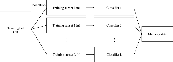
- 也可以叫 bootstrap
- 從訓練資料中隨機抽取樣本(取出後放回，$n \lt N$)
- 訓練多個分類器，每個分類器的權重一致
- 最後用投票方式(Majority vote)得到最終結果
- $h(x) = \frac{1}{K} \Sigma^K_{i=1} h_i(x)$

#### Random forests
- A form of decision tree bagging
- Randomly vary the attribute choices
- We select a random sampling of attributes, and then compute which of those gives the highest information gain
- Every tree in the forest likely will be different extremely randomized trees (ExtraTrees)
- Random forests are resistant to overfitting

### Idea of boosting
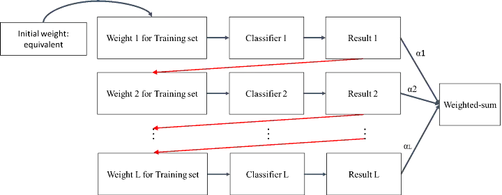
- 將很多個弱的分類器進行合成變成一個強分類器
- 透過將舊分類器的**錯誤資料權重**提高，然後再訓練新的分類器
- 新的分類器會學習到錯誤分類資料的特性，進而提升分類結果
- 對 noise 非常敏感，即如果 data 存在 noise，則該 noise 可能會被放大學習，造成 model 訓練不起來
- Adaboost 為他的改良版

### Idea of stacking
[reference link](https://ithelp.ithome.com.tw/articles/10274009)
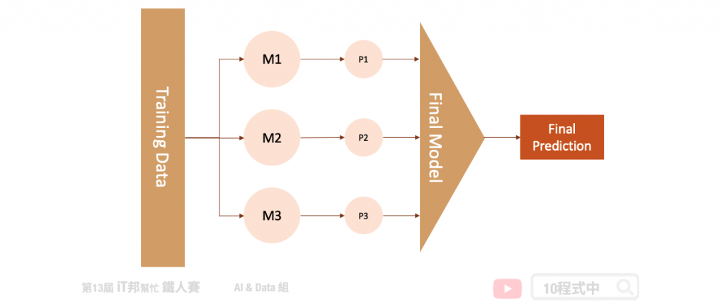
- Combines multiple base models from different model classes trained on the same data
- 結合許多獨立的模型所預測出來的結果，並將每個獨立模型的輸出視為最終模型預測的輸入特徵，最後再訓練一個最終模型
- 每一個模型所訓練出來的預測能力都不同，也許模型一在某個區段的資料有不太好的預測能力，而模型二能補足模型一預測不好的地方
- 將訓練好的模型輸出集合起來(P1、P2、P3、...)，一起訓練最終模型，最後得到預測輸出

### Idea of online learning
- If dataset are not i.i.d.
- 資料間具有次序(例如：歷史事件)
- 或是資料會隨時間更新
- 而我們必須在每個時間點更新預測模型以處理未來的資料
- Useful for applications that involve a large collection of data that is constantly growing
- 例如：像日常生活中使用的詞庫，每個世代都會新增新的用語
- 阿薩斯龍語真的好強