# Asymptotic Time Complexity Tutorial

_Ben Wingerter and Matthew Vavricek_

## What _is_ asymptotic time complexity?: Big Oh, Big Theta, Big Omega

### Big Oh: O
Big O measures the time complexity of the worst case scenario of the the algorithm's execution based on the input. For example, if a sorting algorithm has nested for loops to sort each item, the worst case scenario would be n² if the list was given reverse-sorted.

Note that these bounds apply asymptotically and may be broken at small values.

Below is an image of Big Oh visualized. `k*f(x)`, where `k` is a constant, reprents the upper bound for an algorithm's time complexity.

_*Image Source*: [Khan Academy](https://www.khanacademy.org/computing/computer-science/algorithms/asymptotic-notation/a/big-o-notation)_

### Big Theta: Θ
Big Theta measures the upper _and_ lower bounds of the time complexity of an algorithm's runtime. This is possible by applying constant factors to the big theta value. For example, if an algorithm has a runtime complexity of Θ(3n), then the big theta is Θ(n) because we can apply factors 2 and 4 to make the lower and upper bounds, respectively.

Note that these bounds apply asymptotically and may be broken at small values.

Notice on the graph below that the running time asymptotically falls between n at different factors.

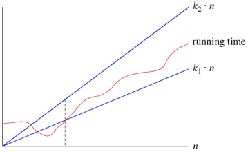
_*Image Source*: [Khan Academy](https://www.khanacademy.org/computing/computer-science/algorithms/asymptotic-notation/a/big-big-theta-notation)_

### Big Omega: Ω
Big Omega measures the asymptotic lower bound of an algorithm's time complexity. In order words, if an algorithm has a Big Omega of `k*f(n)`, or some constant `k` multiplied by the function `f(n)`, it will always have a runtime complexity greater than `k*f(n)`. Naturally, this information isn't always the most helpful because the real time complexity could be significantly greater than the Big Omega.

Like Big Theta, note that this bound applies asymptotically and may be broken at small values.

Below is a simple graphical description of Big Omega.

_*Image Source*: [Khan Academy](https://cdn.kastatic.org/ka-perseus-images/c02e6916d15bacae7a936381af8c6e5a0068f4fd.png)_

## Steps to Analyze a Basic (Iterative) Algorithm
1. **Determine the algorithm's input size based on its parameters.** Algorithm runtime grows as a function of its input, and it's important to identify what changes in input matter and what changes do not. We call the "size" of the input `n`.
* For most algorithms that accept an list, the n is the size of the input list.
* For a function that calculates `x^y`, n is often the value of `y`.
* For a function that calculates `x!`, n is often the value of `x`.
* Once in a while, there will be both an `n` and an `m`. For example, if your algorithm accepts a 2 dimensional array that is _not_ square, the time complexity might be based on both `m` and `n`.
2. **Find the basic operation of the algorithm.** The basic operation is some value that is ran either more or less depending on the size of the input. Good candidates include how many times a multiplication operation is ran or how many times a central if statement is evaluated.
3. **Is the number of times the basic operation is executed only dependent on the input size? If not, worst, average, and best cases must be looked into separately.** For example, if a sorting algorithm runs quicker when the data is already sorted, you must separately define your worst and best case time complexities.
4. **Create a summation showing the number of times the basic operation is executed.** In this step, you find how many times the basic operation is ran based on the input size. It's usually easiest to write it as a summation, or at least for now.
5. **Find a formula to show the operation count and establish the algorithm's order of growth.** In this step, you evaluate any summations and simplify the expression to find the growth function. Once you have this, you can simplify the equation to calculate the algorithm's order of growth (constant, linear, logarithmic, etc.).

### Worked Example: Bubble Sort

static void bubbleSort(int[] arr) {  
    int n = arr.length;  
    int temp = 0;  
    for(int i = 0; i < n; i++){  
        for(int j = 1; j < (n-i); j++){  
            if(arr[j-1] > arr[j]){
                //swap elements  
                temp = arr[j-1];  
                arr[j-1] = arr[j];  
                arr[j] = temp;  
            }
        }  
    }
}

_**Code Source**: https://www.javatpoint.com/bubble-sort-in-java_

#### Step 1: Input size
The input size in this example is easy; it's simply the length of the array `arr`.

#### Step 2: Basic Operation
The basic operation of this algorithm is is the conditional statement `if(arr[j-1] > arr[j]){`. This is the code that gets executed on every iteration of the innermost for loop.

#### Step 3: Is the execution count of the basic operation only dependent on input size?
Yes! The first for loop executes `n` times regardless of the size of n or any other factors. This is because the iterator, `i`, starts at 0 and increments by 1 each iteration that it's less than `n`. The second for loop also executes `n` times. This is because the iterator, `j`, starts at 1 and increments by 1 each iteration that it's less than `n - 1`. Since the inner loop's number of iterations differs from the outer loop's number of iterations by a constant 2, the two loops asymptotically have same execution bounds.

#### Step 4: Summation of Executions

First, set up a summation notation of the number of times the basic operation is executed.


Then continue to simplify the summation based on the summation formulas.






Now since we have the solved summation notation, let's simplify it to find the asymptotic order of growth. We do this by taking the highest order power (n² in this case) and dropping any other terms of equal or lower power. This leaves us with the simplified asymptotic growth of:


## Steps to Analyze a Recursive Algorithm
Often times we need to evaluate the time complexity of a recursive algorithm. The first three steps to analyze the time complexity of a recursive algorithm are the same as analyzing a non-recursive algorithm. Here are all the steps:

1. Determine the algorithm's input size based on its parameters.
2. Find the basic operation of the algorithm.
3. Is the number of times the basic operation is executed only dependent on the input size? If not, worst, average, and best cases must be looked into separately.
4. **Set up a recurrence relation and initial condition for the number of times the basic operation is executed.**
5. **Solve the recurrence equation.** This is usually done with _backsubstitution_, which we will look at later.

## Worked Example: Factorial

static int factorial(int n) {
    if(n == 0) {
        return 1;
    } else {
        return n * factorial(n-1);
    }
}

_**Code Source:** https://www.javatpoint.com/factorial-program-in-java_

#### Step 1: Input size
The input size for this algorithm is the argument `n`, as increasing the size of `n` increases the number of recursive calls required.

#### Step 2: Basic Operation
The basic operation for this function is the multiplication operation in the second return statement.

#### Step 3: Is the execution count of the basic operation only dependent on input size?
In this case, no. Calling `factorial(12)` will always take the same amount of time.

#### Step 4: Set up a recurrence relation and initial condition for the number of times the basic operation is executed.
The algorithm's recurrence relation is defined in two inseparable parts:

1. `F(n)=F(n-1) + 1 for n > 0`
2. `F(0) = 0`

The first line defines the recursive part of the recurrence relation. Since we are counting the number of times the basic operation is executed, we add 1 to the relation on every recursion.

The second line defines the base case of the algorithm. We can see in the code that 1 is returned when the base case is reached (n==0) and the basic operation is not executed. Therefore, we don't add to the recurrence relation when the base case is reached.

#### Step 5: Solve the recurrence equation.
One way to solve recurrence equations is to use **backwards substitution**. This is when we replace the recursive part of the recurence relation with the equation itself and a recursive call one level deeper. Let's take a peek at how this looks.

F(n) = F(n-1) + 1
F(n) = [F(n-2) + 1] + 1

Notice how we replaced the recursive part of the equation (`F(n-1`) with the equation itself and another recurrence (`F(n-2) + 1`). This method makes it easy to see how the recurrence behaves over time and allows us to solve the recurrence relation.

Let's do backwards substitution again.

...
F(n) = ([F(n-3) + 1] + 1) + 1

The behavior of the recurrence should be clear by now. We add 1 to the equation and decrement the substrator of `n` every time we perform backwards substitution. Now let's build a generalized formula to represent this.

F(n) = F(n-i) + i

In this formula, `i` is the number of times we back-substituted.

Now let's use the base case to make a non-recursive version of this. What value of `i` can we use to make the function equal the base case? Let's try `i=n`.

With i=n:
F(n) = F(n-n) + n
F(n) = n

Since `F(n-n)` equals the base case `F(0) = 0`, we made the replacement in the formula.

Therefore, the number of recurrences is n, the size of the input.