---
tags: machine-learning
---
# LeNet-5: Summary and Implementation
<div style="text-align: center">
<img src="https://raw.githubusercontent.com/valoxe/image-storage-1/master/research-paper-summary/alexnet/0.png?token=AMAXSKLOJ332DVKUCQFEDVS6WMFAW">
</div>
>This post is divided into 2 sections: Summary and Implementation.
>
>We are going to have an in-depth review of the [Gradient-Based Learning Applied to Document Recognition](http://vision.stanford.edu/cs598_spring07/papers/Lecun98.pdf) paper which introduces the LeNet-5 architecture.
>
> The implementation uses Keras as framework. For other frameworks implementation, please refer to this [repository](https://github.com/3outeille/Research-Paper-Summary).
>
> Also, if you want to read other "Summary and Implementation", feel free to
> check them at my [blog](https://ferdinandmom.engineer/deep-learning/).

---
# I/ Summary
- ==LeNet is one of the very first convolutional neural networks (CNNs).==
- In the paper, there is several versions of LeNet (LeNet-1, LeNet-4, LeNet-5, Boosted LeNet-4) but here, we are going to focus only on LeNet-5.
Here is its architecture:

- LeNet-5 has:
- 2 **Convolutional** layers.
- 3 **Fully connected** layers.
- 2 **Average pooling** layers.
- **Tanh** as activation function for hidden layer.
- **Softmax** as activation function for output layer.
- 60000 trainable parameters.
- **Cross-entropy** as cost function
- **Gradient descent** as optimizer.
- LeNet-5 is:
- trained on MNIST dataset (60000 training examples).
- trained over 20 epochs.
- LeNet-5 is expected to:
- converge after 10–12 epochs.
- have an error rate of 0.95% on test set. (Using accuracy as metric)
# II/ Implementation
- We will use a simpler version of the LeNet-5 than the one described in the paper. For example, computation on average pooling layers described in the paper are slightly more complex than usual.
- The implementation is divided as follow:
1. Import libraries
2. Loading dataset
3. Data preprocessing
4. Data visualization
5. Architecture build
6. Training
7. Evaluating
## 1. Import libraries
```python
from tensorflow.keras import Sequential
from tensorflow.keras.layers import Conv2D, AveragePooling2D, Flatten, Dense
from tensorflow.keras.losses import CategoricalCrossentropy
import numpy as np
import matplotlib.pyplot as plt
import tensorflow as tf
%matplotlib inline
```
## 2. Loading dataset
```python
(X_train, y_train), (X_test, y_test) = tf.keras.datasets.mnist.load_data()
X_val, y_val = X_train[55000:, ..., np.newaxis], y_train[55000:]
X_train, y_train = X_train[:55000, ..., np.newaxis], y_train[:55000]
X_test = X_test[..., np.newaxis]
print("Image Shape: {}".format(X_train[0].shape), end = '\n\n')
print("Training Set: {} samples".format(len(X_train)))
print("Validation Set: {} samples".format(len(X_val)))
print("Test Set: {} samples".format(len(X_test)))
```
If everything went well, you should get the following output:
```python
Image Shape: (28, 28, 1)
Training Set: 55000 samples
Validation Set: 5000 samples
Test Set: 10000 samples
```
## 3. Data preprocessing
Firstly, check if your ~/.keras/keras.json file has the following line:
```
"image_data_format": "channels_first"
```
If not, replace it to:
```
"image_data_format": "channels_last
```
Now, we need to:
- reshape the image into a 32x32x1 shape.
- normalize our dataset.
### Reshape the image into a 32x32x1 shape
```python
# Pad images with 0s
X_train = np.pad(X_train, ((0,0),(2,2),(2,2),(0,0)), 'constant')
X_val = np.pad(X_val, ((0,0),(2,2),(2,2),(0,0)), 'constant')
X_test = np.pad(X_test, ((0,0),(2,2),(2,2),(0,0)), 'constant')
print("Updated Image Shape for: ", end='\n\n')
print("-Training set: {}".format(X_train.shape))
print("-Validation set: {}".format(X_val.shape))
print("-Test set: {}".format(X_test.shape))
```
### Normalize our dataset
```python
# Normalization.
X_train, X_val, X_test = X_train/float(255), X_val/float(255), X_test/float(255)
X_train -= np.mean(X_train)
X_val -= np.mean(X_val)
X_test -= np.mean(X_test)
```
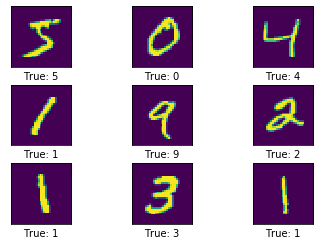
## 4. Data visualization
Let's visualize some pictures. Here is how it looks:

## 5. Architecture build
Following the Figure 2 above, here is LeNet-5 architecture in Keras.
```python
def LeNet_5():
model = Sequential()
# C1: (None,32,32,1) -> (None,28,28,6).
model.add(Conv2D(6, kernel_size=(5, 5), strides=(1, 1), activation='tanh', input_shape=(32,32,1), padding='valid'))
# P1: (None,28,28,6) -> (None,14,14,6).
model.add(AveragePooling2D(pool_size=(2, 2), strides=(2, 2), padding='valid'))
# C2: (None,14,14,6) -> (None,10,10,16).
model.add(Conv2D(16, kernel_size=(5, 5), strides=(1, 1), activation='tanh', padding='valid'))
# P2: (None,10,10,16) -> (None,5,5,16).
model.add(AveragePooling2D(pool_size=(2, 2), strides=(2, 2), padding='valid'))
# Flatten: (None,5,5,16) -> (None, 400).
model.add(Flatten())
# FC1: (None, 400) -> (None,120).
model.add(Dense(120, activation='tanh'))
# FC2: (None,120) -> (None,84).
model.add(Dense(84, activation='tanh'))
# FC3: (None,84) -> (None,10).
model.add(Dense(10, activation='softmax'))
# Compile the model
model.compile(loss='sparse_categorical_crossentropy', optimizer='sgd', metrics=['accuracy'])
return model
```
## 6. Training
Let's train and save our model.
```python
history = model.fit(X_train, y_train, validation_data=(X_val, y_val), epochs=20)
# Save the model.
model.save("lenet5_model.h5")
```
## 7. Evaluating
Now, let's test our model.
```python
# Restore the model.
model = tf.keras.models.load_model('lenet5_model.h5')
# Make prediction.
predictions = model.predict(X_test)
# Retrieve predictions indexes.
y_pred = np.argmax(predictions, axis=1)
# Print test set accuracy.
print('Test set error rate: {}'.format(np.mean(y_pred == y_test)))
# Plot some examples with model predictions.
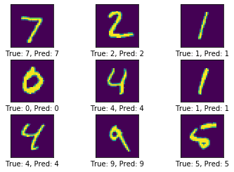
print('\nSome correct classification:')
plot_example(X_test, y_test, y_pred)
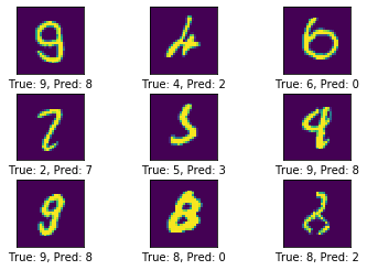
print('\nSome incorrect classification:')
plot_example_errors(X_test, y_test, y_pred)
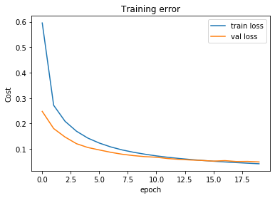
# Plot training error.
print('\nPlot of training error over 20 epochs:')
plt.title('Training error')
plt.ylabel('Cost')
plt.xlabel('epoch')
plt.plot(history.history['loss'])
plt.plot(history.history['val_loss'])
plt.legend(['train loss', 'val loss'], loc='upper right')
plt.show()
```
We should get the following output:
```python
Test set error rate: 0.9837
```
Some correct classification:

Some incorrect classification:

Plot of training error over 20 epochs:
