# Recognization Using SVM,Random Forest and NN.
## Data Set 下載
[sklearn 內建資料集](https://scikit-learn.org/stable/datasets/index.html)
[外部開源資料集](https://www.kaggle.com/)
## Google Colaboratory
[Google Colab](https://colab.research.google.com)
Python具有簡潔高效、可移植性強、龐大的標準庫等優勢,因此被廣泛使用於機器學習上。
常用模組:
-numpy:主要用在資料處理上,能快速操作多重維度的陣列
ex: import numpy as np
-pandas:將大量資料透過結構化進行前處理以及整合的動作
ex: import pandas as pd
-matplotlib.pyplot:將資料視覺化,將數據以圖像的方式呈現出來
ex: import matplotlib.pyplot as plt
-scikit-learn(SKlearn):專門用來時作機器學習以及資料採礦,有預測模型、分群等多種功用
ex1: from sklearn.model_selection import train_test_split
ex2: from sklearn.neighbors import KNeighborsClassifier
**<font color = "red">**※Python不用打分號!**</font>**
## 實作
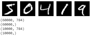
[MNIST 手寫數字圖片資料](http://yann.lecun.com/exdb/mnist/)
以digits dataset為例,手寫數字辨認非常適用於機器學習入門,資料總筆數為70000筆(train data:60000筆、test data:10000筆),每一筆資料有28X28個像素。
```pyhton=
import numpy as np
import keras
import tensorflow
from keras.datasets import mnist
from matplotlib import pyplot as plt
%matplotlib inline
(x_train, y_train), (x_test, y_test) = mnist.load_data()
fig = plt.figure()
for i in range(5):
fig.add_subplot(1, 5, i + 1) #新增子圖 (顯示區中有幾列 , 有幾行 , 第幾個圖形)
plt.imshow(x_train[i], cmap=plt.get_cmap('gray')) #圖像繪製 (要畫的圖象 , cmap=顏色)
plt.axis('off') #是否顯示座標尺
plt.show()
x_train = np.reshape(x_train, [-1, 784]) / 255.0
x_test = np.reshape(x_test, [-1, 784]) / 255.0
print(x_train.shape)
print(y_train.shape)
print(x_test.shape)
print(y_test.shape)
```
## SVM 原理
- 尋找一個分離超平面,使得它到各分類的平均距離是最大的


- 調整參數'C'和'gamma'的影響:

## SVM 測試
```python=
def get_data(x,y,k): #從60000筆資料中隨機得想要的幾筆資料
rand_arr = np.arange(x.shape[0])
np.random.shuffle(rand_arr)
a = x[rand_arr[0:k]]
b = y[rand_arr[0:k]]
return a,b
x1_train,y1_train = get_data(x_train,y_train,3000)
x1_test,y1_test = get_data(x_test,y_test,3000)
print(x1_train.shape)
print(y1_train.shape)
print(x1_test.shape)
print(y1_test.shape)
from sklearn.svm import SVC
clf = SVC(kernel='rbf',gamma=1,C=1)
clf.fit(x1_train,y1_train)
score = clf.score(x1_test,y1_test)
print(score)
```
將準確率提高至0.94以上吧!
## Random Forest 原理
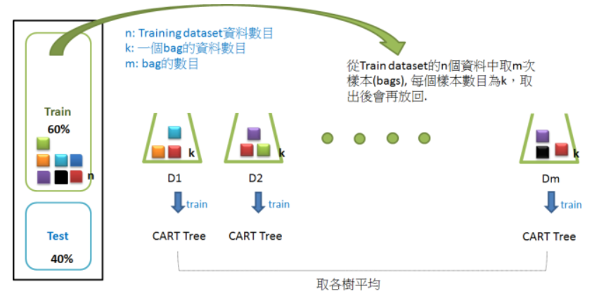
Random Forest,結合多顆CART樹(CART樹為使用GINI算法的決策樹),並加入隨機分配的訓練資料,以大幅增進最終的運算結果。
## Random Forest 測試
```pyhton=
from sklearn.ensemble import RandomForestClassifier
from sklearn.model_selection import train_test_split
clf = RandomForestClassifier(n_estimators=1,max_depth=1, random_state=1)
clf = clf.fit(x_train, y_train)
print(clf.score(x_test,y_test))
```
將準確率提高至0.971以上吧!
---
## NN 原理
[快速瀏覽](https://medium.com/@intheblackworld/deep-learning-tutorial-%E5%BF%83%E5%BE%97-b1f7f84a497d)

## NN 測試
keras.Model
Keras 提供一些模型基底,可以從這些基底開始,設計自己的神經網路模型。請參考 About Keras models 了解 Keras 模型。
```python
from keras.models import Sequential
model = Sequential()
```
一個神經網路模型可以呼叫 model.add() 增加隱藏層,Keras 提供許多隱藏層的實作,讓你可以專注於隱藏層的選擇策略以及參數調整。常見的有 Dense (全連結層)與 Dropout 等等,可以透過 activation 參數設定該層的激活函數。可以呼叫 model.summary() 檢視設計好的模型。請參考 About Keras layers 了解 Keras 層,參考 Activations 了解激活函數。
```python
from keras.layers import Dense
model.add(Dense(16, input_dim=784, activation='sigmoid'))
model.add(Dense(1, activation='sigmoid'))
model.summary()
```
模型設計完需要呼叫 compile() 編譯之後才能使用,在編譯時可以設定損失函數(loss)、評估標準(metrics)以及等優化器(optimizer)參數。請參考 compile() 了解編譯,參考 Losses 了解損失函數,參考 Optimizers 了解優化器。
```python
model.compile(loss='binary_crossentropy', metrics = ['accuracy'], optimizer='adam')
```
編譯完成的模型可以呼叫 fit() 訓練模型,訓練時需給定訓練資料(prepared.x_train 與 prepared.y_train)並設定 batch_size、epochs 等參數。請參考 fit()。
```python
model.fit(prepared.x_train, prepared.y_train, batch_size=10000, epochs=1, verbose=1)
```
訓練完成的模型可以呼叫 predict() 進行預測。請參考 predict()。
```python
y_pred = model.predict(prepared.x_test)
```
或是直接呼叫 evaluate() 評估效能。請參考 evaluate()。
```python
score = model.evaluate(prepared.x_test, prepared.y_test)
print('loss: %f, accuracy: %f' % (score[0], score[1]))
```
### 測試
[activations function](https://keras.io/activations/)
[losses function ](https://keras.io/losses/) #輸出結果與目標結果的差距
[optimizers](https://keras.io/optimizers/) #最小化loss function
[metrics](https://keras.io/metrics/) #評估指標 Accuracy、Precision、Recall或其他指標
[fit]()
由於損失函數可能是一個非常複雜的曲線,或逼近最佳解的幅度過小,都會使得優化速度過慢或不穩定,所以我們要限制求解的最大訓練週期(Epochs),以免跑不完。另外,梯度下降若每次都使用全部資料求斜率,可能會花費太多時間,所以通常會採用隨機抽樣,分批求解,batch_size就是指定一批要抽多少樣本。
```python
import numpy as np
from keras.models import Sequential
from keras.layers import Dense
from keras.datasets import mnist
from keras.utils import to_categorical
(x_train, y_train), (x_test, y_test) = mnist.load_data()
x_train = np.reshape(x_train, [-1, 784])
x_test = np.reshape(x_test, [-1, 784])
y_train = to_categorical(y_train, num_classes=10)
y_test = to_categorical(y_test, num_classes=10)
# try
model = Sequential()
model = Sequential()
model.add(Dense(100, activation='sigmoid'))
model.add(Dense(10, activation='softmax'))
model.compile(loss='categorical_crossentropy', optimizer='sgd', metrics=['accuracy'])
model.fit(x_train, y_train, batch_size=200, epochs=10, validation_split=0.2)
score = model.evaluate(x_test, y_test)
print('loss: %f, accuracy: %f' % (score[0], score[1]))
```
 Sign in with Wallet
Connect another wallet
Sign in with Wallet
Connect another wallet