# Kung-Fu OpenCV

## Image Quantization
This is useful to have an easier color filter intuition.

Code:

#==========change to depth 6 (8 bpp) rgb222 {FASTER}
img_tmp=input_img.copy() # Copy input image
con1 = np.where(img_tmp<64,0,img_tmp)
con2 = np.where((con1>=64) & (con1<128),64,con1)
con3 = np.where((con2>=128) & (con2<192),128,con2)
con4 = np.where(con3>192,255,con3)

## Hough circles
[Explanation:](https://www.youtube.com/watch?v=Ltqt24SQQoI)
1. Hough circle will find points that is alligned into a circle
2. Edge image is needed
3. Specific Radius is needed
4. Draw circle in every points of edge. Put it on 'accumulator image space'
5. What we got is many circles
6. The intersection of this circles are the center of a circle we want in that radius
7. OpenCV uses range of radius instead of one specific radius

Steps:
1. create edge image using:
a. [Sobel operator](https://docs.opencv.org/2.4/doc/tutorials/imgproc/imgtrans/sobel_derivatives/sobel_derivatives.html)
b. [Canny edge detection](https://docs.opencv.org/trunk/da/d22/tutorial_py_canny.html) `cv.Canny(img,100,200)`
2. [Apply](https://docs.opencv.org/2.4/modules/imgproc/doc/feature_detection.html?highlight=houghcircles#houghcircles) `arr_cir = cv.HoughCircles(img_edges, cv.HOUGH_GRADIENT,1,50, param1=100,param2=15,minRadius=20,maxRadius=40)`
a. The result is positions and radius of each circle
b. `1` is accumulator image ratio. `1` means accumulator image is the same with the souce image
c. `50` is the distance treshold of one circle to another
d. `param1` the higher threshold of the two passed to the Canny() edge detector (the lower one is twice smaller)
e. `param2` is argument for circularity confidence. It is like a circularity treshold from the algorithm
f. `minRadius` – Minimum circle radius.
g. `maxRadius` – Maximum circle radius.
3.

## Blob filter

**B**inary **L**arge **OB**ject

Blob information
1. location
2. size

Filters:
1. size
2. circularity
3. convexity
4. etc

[The sauce](https://www.learnopencv.com/blob-detection-using-opencv-python-c/)

NOTES
> Datected blobs are in black color

Main alghorithm:
1. Create binary image
2. Create blob parameter `cv2.SimpleBlobDetector_Params()`
3. Create detector `cv2.SimpleBlobDetector_create(params)`
4. Perform and extract the keypoints `keypoints = detector.detect(im)`

CODE:

# Setup SimpleBlobDetector parameters.
params = cv2.SimpleBlobDetector_Params()

# Change thresholds
params.minThreshold = 10;
params.maxThreshold = 200;

# Filter by Area.
params.filterByArea = True
params.minArea = 1500

# Filter by Circularity
params.filterByCircularity = True
params.minCircularity = 0.1

# Filter by Convexity
params.filterByConvexity = True
params.minConvexity = 0.87

# Filter by Inertia
params.filterByInertia = True
params.minInertiaRatio = 0.01

# Create a detector with the parameters
ver = (cv2.__version__).split('.')
if int(ver[0]) < 3 :
	detector = cv2.SimpleBlobDetector(params)
else : 
	detector = cv2.SimpleBlobDetector_create(params)
    
# Detect blobs
keypoints = detector.detect(im)
# Draw detected blobs as red circles.
# cv2.DRAW_MATCHES_FLAGS_DRAW_RICH_KEYPOINTS ensures the size of the circle corresponds to the size of blob
im_with_keypoints = cv2.drawKeypoints(im, keypoints, np.array([]), (0,0,255), cv2.DRAW_MATCHES_FLAGS_DRAW_RICH_KEYPOINTS)

## Finding a contour
Finds [contours](https://docs.opencv.org/2.4/doc/tutorials/imgproc/shapedescriptors/find_contours/find_contours.html) in a binary image.
There are many algorithm that can be applied after finding contour

Steps:
1. Create binary image
2. [Apply](https://docs.opencv.org/2.4/modules/imgproc/doc/structural_analysis_and_shape_descriptors.html?highlight=boundingrect#findcontours)

image, contours, hierarchy	=	cv.findContours(	image, mode, method[, contours[, hierarchy[, offset]]]	)

3. `contours` is array containing array of contour (connected points)
4. `hierarchy` it's a contour hierarchy if there are contours inside contour. `[Next, Previous, First_Child, Parent]`
5. Hierarchy :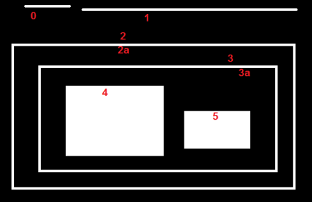 
6. For each i-th contour `contours[i]` , the elements `hierarchy[i][0]`, `hiearchy[i][1]`, `hiearchy[i][2]`, and `hiearchy[i][3]` are set to 0-based indices in contours of the next and previous contours at the same hierarchical level

## Approximate polygon / polygon approximation
[Documentation](https://docs.opencv.org/2.4/modules/imgproc/doc/structural_analysis_and_shape_descriptors.html?highlight=boundingrect#approxpolydp)



OpenCV uses [Ramer-Douglas-Peucker](https://www.youtube.com/watch?v=nSYw9GrakjY&t=1383s)

Steps:
1. Obtain Contour
2. Apply `cv2.approxPolyDP(curve, epsilon, closed[, approxCurve])`

## Find a bounding box
[Calculates the up-right bounding rectangle of a point set.](https://docs.opencv.org/2.4/modules/imgproc/doc/structural_analysis_and_shape_descriptors.html?highlight=boundingrect#boundingrect)

Steps:
1. Obtain contour
2. Apply `cv.BoundingRect(points, update=0)`
3. `points` can be contours

## Calculate area of a contour
[Calculates a contour area.](https://docs.opencv.org/2.4/modules/imgproc/doc/structural_analysis_and_shape_descriptors.html?highlight=boundingrect#contourarea)
The function computes a contour area. Similarly to [moments()](https://docs.opencv.org/2.4/modules/imgproc/doc/structural_analysis_and_shape_descriptors.html?highlight=boundingrect#moments), the area is computed using the Green formula. Thus, the returned area and the number of non-zero pixels, if you draw the contour using `drawContours()` or `fillPoly()` , can be different. Also, the function will most certainly give a wrong results for contours with self-intersections.

Steps:
1. Create contour
2. Apply `cv.ContourArea(contour, slice=CV_WHOLE_SEQ)`

## Convex Hull
[Finds the convex hull of a point set.](https://docs.opencv.org/2.4/modules/imgproc/doc/structural_analysis_and_shape_descriptors.html?highlight=boundingrect#convexhull)

Steps:
1. Create contour
2. `cv.ConvexHull2(points, storage, orientation=CV_CLOCKWISE, return_points=0)`

## Convexity defects
[Finds the convexity defects of a contour.](https://docs.opencv.org/2.4/modules/imgproc/doc/structural_analysis_and_shape_descriptors.html?highlight=boundingrect#convexitydefects)

Steps:
1. Create contour
2. `cv2.convexityDefects(contour, convexhull[, convexityDefects])`
3. The result is array containing informations of each defects

struct CvConvexityDefect
{
   CvPoint* start; // point of the contour where the defect begins
   CvPoint* end; // point of the contour where the defect ends
   CvPoint* depth_point; // the farthest from the convex hull point within the defect
   float depth; // distance between the farthest point and the convex hull
};

## Put a color into the blob and find contour

This will be usefull for removing unwanted blobs or highlighting wanted blob. The wanted blob can be turned into white and the other to be black. This will form a mask for later process.

Main alghorithm:
1. Create binary image `cv.threshold()`
2. Find Contours `cv.findContours()`
3. Put color in the contour`cv.drawContours()`
4. $-1$ in the parameter means block color

[The sauce](https://docs.opencv.org/3.4/d2/dbd/tutorial_distance_transform.html)

CODE

# Threshold to obtain the peaks
# This will be the markers for the foreground objects
# dist image is binary image

_, dist = cv.threshold(input_img, 180, 255, cv.THRESH_BINARY)
# Dilate a bit the dist image
kernel1 = np.ones((3,3), dtype=np.uint8)
dist = cv.dilate(dist, kernel1)
# Create the CV_8U version of the dist image
# It is needed for findContours()
dist_8u = image.astype('uint8')
# Find total markers
_, contours, _ = cv.findContours(dist_8u, cv.RETR_EXTERNAL, cv.CHAIN_APPROX_SIMPLE)
# Create the marker image for the watershed algorithm
markers = np.zeros(dist.shape, dtype=np.int32)
# Draw the foreground markers
for i in range(len(contours)):
    cv.drawContours(markers, contours, i, (i+1), -1)
#-1 is the block fill 

## Opening and closing

Opening and closing a blob.
[The sauce](https://opencv-python-tutroals.readthedocs.io/en/latest/py_tutorials/py_imgproc/py_morphological_ops/py_morphological_ops.html)

Steps:
1. Create binary image
2. Ctreate kernel, the size does matter
3. Apply `morphologyEx()`

Opening:
CODE:

kernel = np.ones((5,5),np.uint8)
opening = cv2.morphologyEx(img, cv2.MORPH_OPEN, kernel)

Closing:

CODE:

kernel = np.ones((5,5),np.uint8)
opening = cv2.morphologyEx(img, cv2.MORPH_CLOSE, kernel)

## Fill color paint style

[The sauce](https://www.learnopencv.com/filling-holes-in-an-image-using-opencv-python-c/)

This function fills a connected component with color.
To apply the function, choose the location, and color between $\{0,\dots,255\}$
Another way is to use findContours to find the contours and then fill it in using drawContours.

Steps:
1. Create binary image
2. Choose a point inside a blob
3. Choose a color
4. Apply `cv2.floodFill()`

CODE:

# Floodfill from point (0, 0) with value 255
cv2.floodFill(im_floodfill, mask, (0,0), 255)

## Distance transform and find maximum inscribed circle

This algorithm is usefull for findingthe middle point and its clossest distance to the edge.
The result is maximum inscribed circle.
It can be used for watrshed classification.

[Image before](https://docs.opencv.org/3.4/d2/dbd/tutorial_distance_transform.html)
Image after distance transform

[Maximum inscribed circle](https://au.mathworks.com/matlabcentral/fileexchange/30805-maximum-inscribed-circle-using-distance-transform)

Steps:
1. Create binary image
2. Apply `cv.distanceTransform()`

CODE:

dist = cv.distanceTransform(input_binary_image, cv.DIST_L2, 3)

## Grab Cut or Graph Cut
May be the name is wrong.
And I still don't know how it works, but it is amazing.

[Sauce](https://codeloop.org/python-opencv-grabcut-foreground-detection/)

## Another Kung-Fu

Formfactor = 4 pi Area / Perimeter^2
Roundness = 4 Area / (pi Max-diam^2)
Aspect ratio = Max-diam / Min-diam
Curl = max caliper diam / fiber length
Convexity = Convex Perimeter / Perimeter
Solidity = Area / Convex Area
Compactness = sqrt ( 4 * area / pi) / max diameter
Modification ratio = inscribed diameter / max diameter
Extent = Net Area / area of bounding rectangle

###### tags: Programming