# Dietary Pattern Clustering with diabetes

- Presentation for RHINO2021(2021.08.17 ~ 19), Young Jin Kim([e-mail])
- ==If you want to ++more discuss++, please redirect [**here**](https://hackmd.io/@kssZJxcVQluDOozZSnOuSg/HJfY6SQxK)==
- Every image can expand with ++_<Right click> + `Open image in new tab`_++

###### tags: `network` `clustering` `modularity` `dietary pattern` `diabetes` `manifold learning` `auto encoder`

[TOC]

## Highlight

- We find more healthy/critical dietary pattern for diabetes.
- Daily food intake follows log-normal distribution.
- Modularity-based clustering catch the micro difference of dietary pattern.
- Machine learning algorithms (including neural network model: Auto Encoder and Variational Auto Encoder) don't catch the micro difference and just learned global pattern (AE).

## Introduction

Diabetes is one of the most prominent diseases in the 21st century. Not only are there statistical surveys with prevalence rates of around 10% in the world including Korea. The dietary pattern is one of the important factors for the progress of diabetes. We want to find specific dietary patterns more critical to diabetes in KoGES data. We apply the network clustering method and manifold learning like the autoencoder to dietary patterns of Korean and find some micro clusters more critical or healthy for diabetes.

## Data: KoGES

### Korean Genome and Epidemiology Study

KoGES(Korean Genome and Epidemiology Study) is one of biggest data-driven bio-project in Korea [^1]. The KoGES collects epidemiological data and biospecimen, such as blood, urine, and genome from large scale cohort of 40-69 years old by conducting **medical examination** and **health survey**.

In the KoGES, we use one of population-based study "Ansan and Ansung Cohort"

- Men and women living in Ansan (industrialized community) and Ansung (rural area) aged 40–69 years
- 10,030 baseline participants (Ansan: 5,012 Ansung: 5,018)
- 8th follow-up from 2001 to 2018 per 2 years

### Dietary pattern

In this study, we only focus on the dietary pattern. Our hypothesis is it like a famous movie quotes. We suppose that the dietary pattern embraces ones eating, living, and exercise pattern and other all of ones life to exaggerate.

> "Manners maketh man" [name=Harry, Kingsman(2015)]

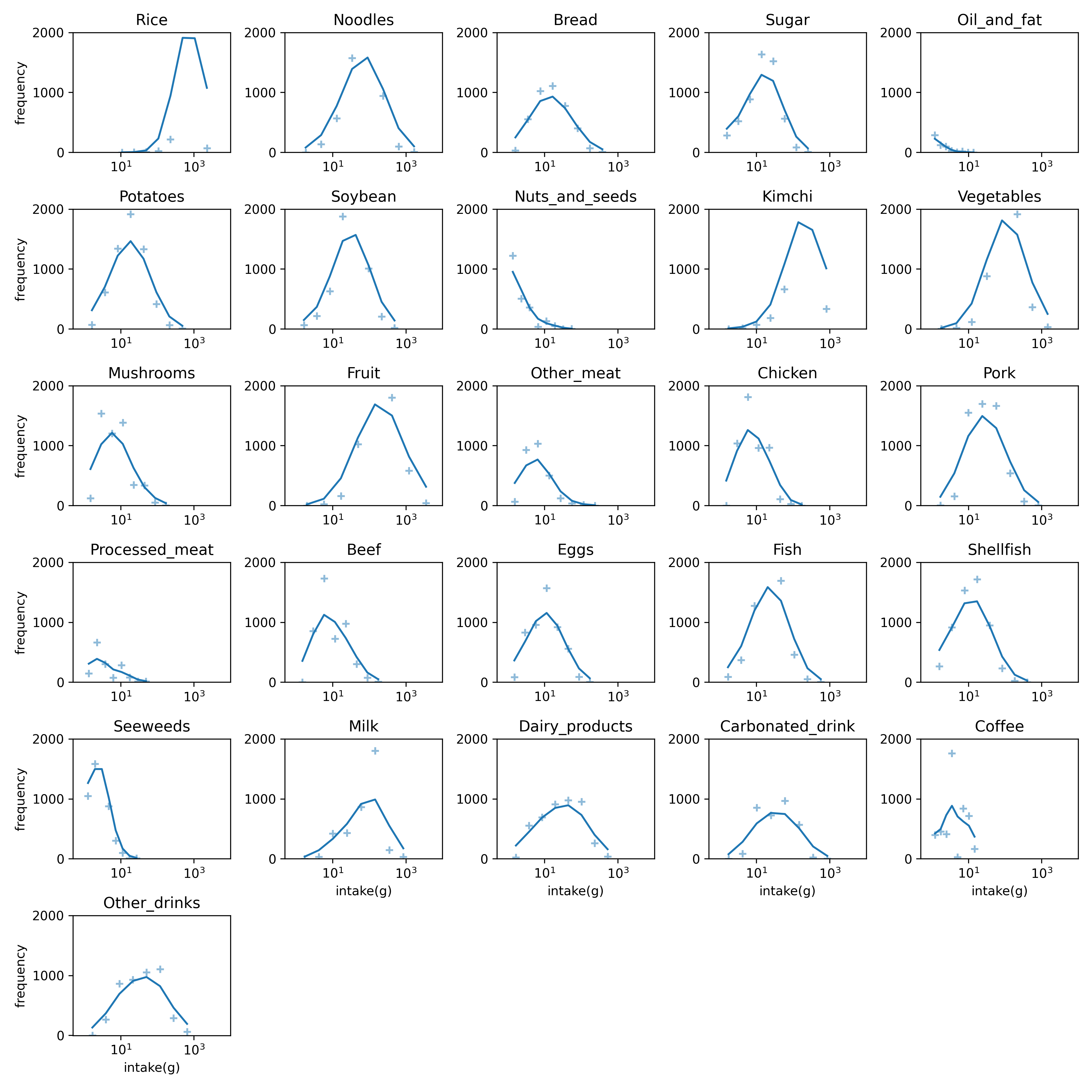
The dietary pattern of the KoGES is made by a survey of the intake and frequency (average in last a year) of the typical food in Korea. The typical foods in survey are 100s. We grouped these foods to 26 represent food groups[^2]. We estimate daily intake of each food group by the survey and make dietary pattern of each patient.

|  |
| :----------------------------------------------------------: |
| **Figure1**. Food distribution in the baseline. The intake of each food follow a log-normal distribution. The number of bins is 9 and the frequency line is smoothen with $\sigma=1$​.​ The non-intake food isn't counted. |

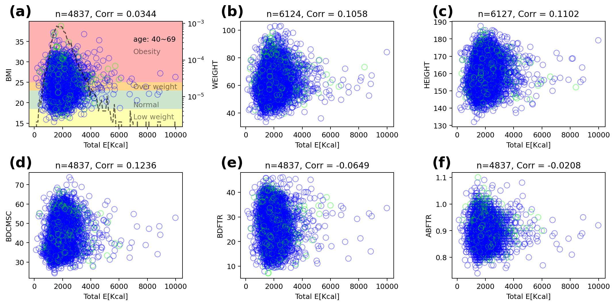
The KoGES dataset contains some anthropometric data like Body Mass Index(BMI). Figure 2 shows correlations between total energy and anthropometric data, and the correlations are not significant. The total energy is estimated using the dietary pattern and national standard ingredients of food. So, there are anomaly data point (almost zero-calories or nearby 10,000 Kcal) in estimated total energy using survey.

|  |
| ------------------------------------------------------------ |
| **Figure 2**. The correlation of total energy and anthropometric data. The blue(green) circle is normal subject (diabetes mellitus) and black dashed line is frequency of total energy. (d-f) show some results from Inbody(3.0) - **(d)** BDCMSC(amount of muscle), **(e)** BDFTR(body fat ratio), and **(f)** ABFTR(abdomen fat ratio). |

### Definition of diabetes and prediabetes

Incident Diabetes Mellitus (DM) was defined as self-reported physician-diagnosed diabetes and/or subjects with current treatment for diabetes (i.e. oral agents and/or insulin) and/or current American Diabetes Association (ADA) guidelines: a fasting glucose concentration ≥126mg/dL or a post 2-h glucose during 75g oral glucose tolerance test (OGTT) of ≥200mg/dL, or HbA1c of ≥6.5% [^3]. Subjects with prediabetes were also defined by ADA guidelines: the presence of impaired fasting glucose (IFG) and/or impaired glucose tolerance (IGT) and/or HbA1c 5.7-6.4%. IFG is defined as fasting glucose concentration between 100 and 125mg/dL [^4][^5] and IGT as post 2-h glucose during 75g OGTT levels between 140 and 199mg/dL [^4].

### CONSORT flow diagram

|  |
| :----------------------------------------------------------: |
| **Figure 3**. CONSORT flow diagram. We focus on 6,127 non-diabetes subjects in baseline. 12.8% of these subjects got the diabetes in outcome. |

## Method

### Modularity-based clustering

Modularity is a measurement of network structure. It means strength of module structure (group, community, or cluster). A network with high modularity has dense internal connection in each module and sparse external connection. The modularity $Q$​ defined the relative internal edge density versus given random network.
$$
Q = \dfrac{1}{w} \sum_{i,j}\left(A_{ij} - \gamma \dfrac{d_id_j}{w}\right)\delta_{c_i,c_j}
$$
where

- $c_i$ is the cluster of node $i$,
- $d_i$ is the weight of node $i$,
- $w = 1^TA1$ is the total weight of the graph,
- $\delta$ is the Kronecker symbol,
- $\gamma$ is the resolution parameter.

We use Louvain algorithm to measure modularity [^6]. This algorithm has advantage with fast calculation and hierarchy. The algorithm merge a node set in a community to a node in each step, so it can obtain the hierarchy of given network. We user a python package `scikit-network` to use Louvain algorithm [^7].

## Result

### Hierarchical cluster

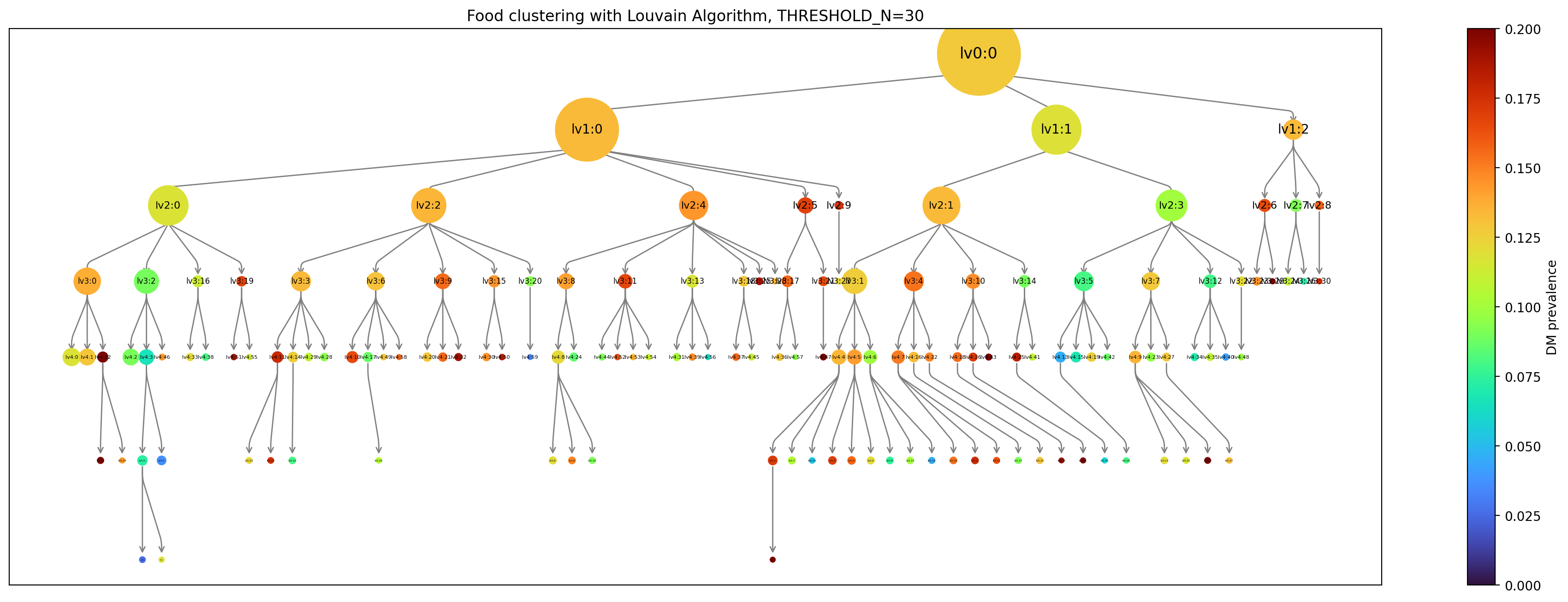
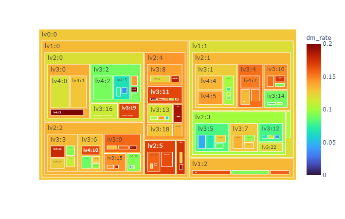
We obtain hierarchy structure of clusters using Louvain algorithm. In low level (lv1), there is not obvious risky/healthy cluster. In more deep stage (lv2~), risky/healthy cluster is appeared (Figure 4).

|  |
| :----------------------------------------------------------: |
| **Figure 4**. Hierarchy of clustering with Louvain algorithm. Each node means a cluster in hierarchy upto lv6. The cluster appears when it contains more than 30 subjects. The size of node means number of cluster and color means diabetes mellitus prevalence(%) in future. The total subject is 6,127. |

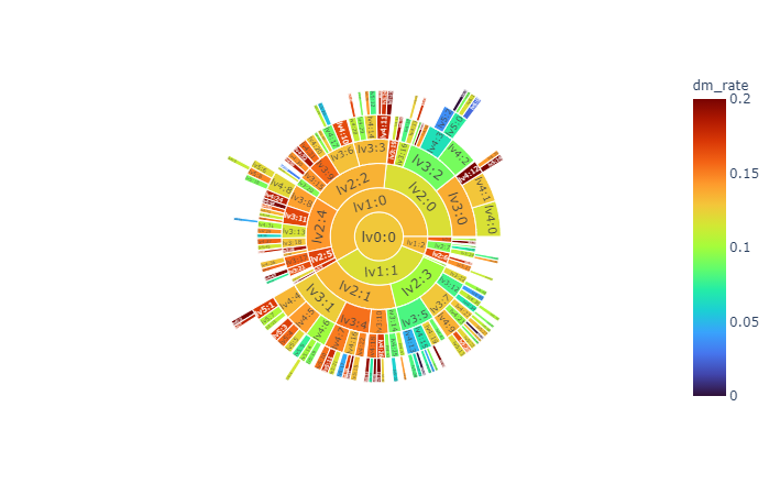
- More interactive visualizations

|  |  |
| :----------------------------------------------------------: | :----------------------------------------------------------: |
| [sunburst](https://kimyoungjin06.github.io/home/presentation/RHINO2021/sunburst.html) | [treemap](https://kimyoungjin06.github.io/home/presentation/RHINO2021/treemap.html) |

### Details in micro clusters (lv4)

We examine typical micro clusters in lv4. The characteristic dietary pattern appear in micro(small) cluster remarkably. Figure 5 shows dietary patterns of top-3 risky/healthy clusters in lv4. The original data doesn't show any correlation with DM, but the obtained cluster by dietary pattern has significant difference in DM prevalence. It means the modularity-based hierarchical clustering understand the micro information underlying structure of similarity network of dietary pattern. Figure 6 shows the major nutrition intake of each cluster. The DM subjects are not 'heavy eater', rather than they eat less. Especially, they mainly eat carbohydrate.

#### Dietary patterns of typical micro cluster

|  |
| :----------------------------------------------------------: |
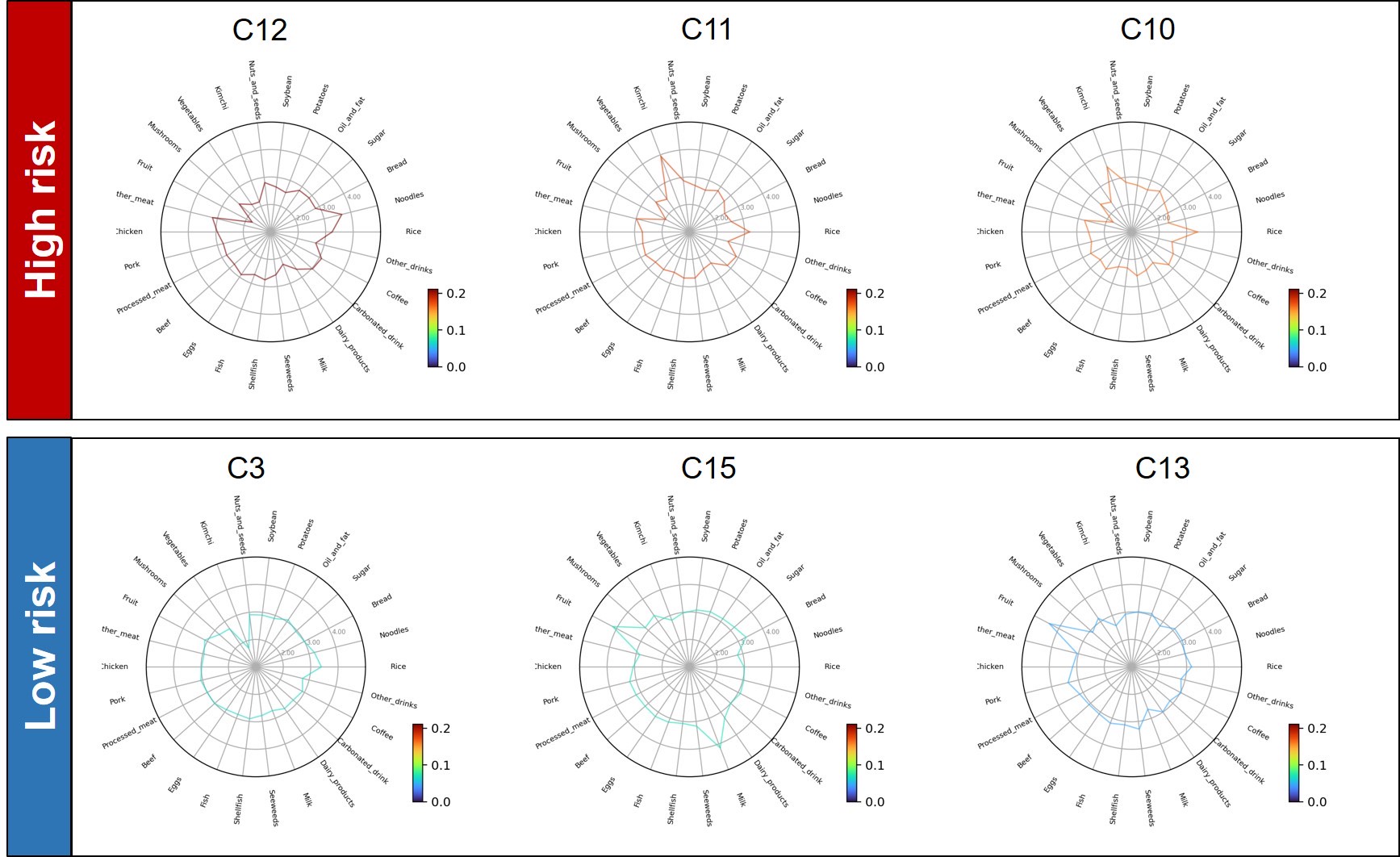| **Figure 5**. Dietary patterns of typical micro cluster in lv4. The color means diabetes mellitus prevalence. Each food score means standardized score with $m=3, \sigma=1$. These clusters are top-3 risky/healthy clusters contains more than 100 subjects. |

#### Major nutrition intake

|  |
| :----------------------------------------------------------: |
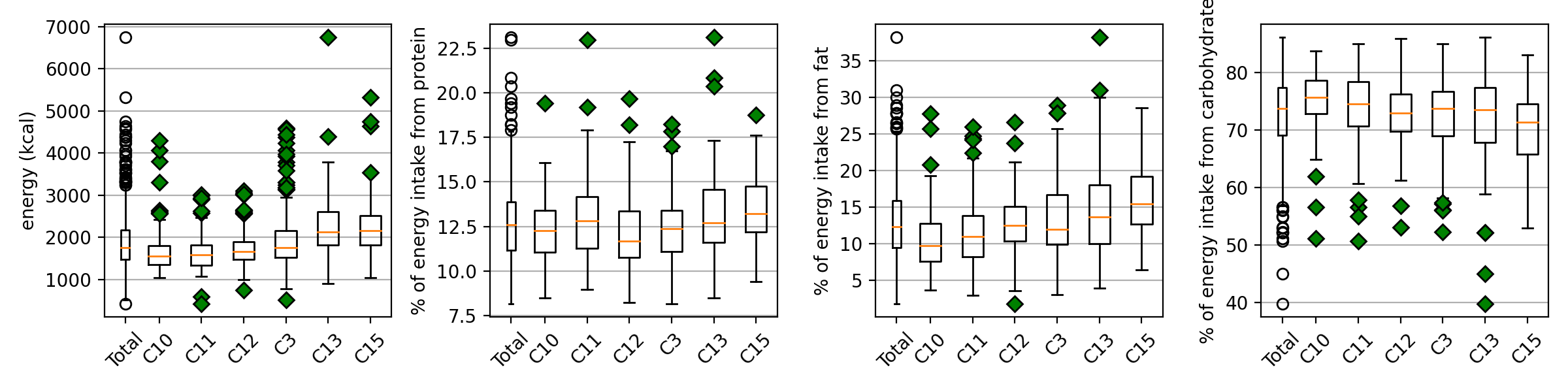| **Figure 6**. Major nutrition intake. The healthy (C3, C13, and C15) clusters absorb more calories (especially the form of fat), and the risky clusters absorb more energy from carbohydrate. \*\*The whisker is 1.5. |

### Manifold learning: Auto Encoder

Auto Encoder is one of manifold learning model to reduce dimension using neural network. The AE is designed to find hidden structure of data. The AE has two main parts: encoder and decoder. The encoder maps the original data $x$ to code $h$ (reduced hidden structure) and the decoder maps the code $h$ to re-construction of input $x'$. If $h$ contains all information of original data, it can construct $x'$ from $h$.

We design structure of the AE with 4 hidden layers (26-12-6-**3**-6-12-26). The reduced dimension is 3. In our study, the AE just learned only global information.

|  |
| :----------------------------------------------------------: |
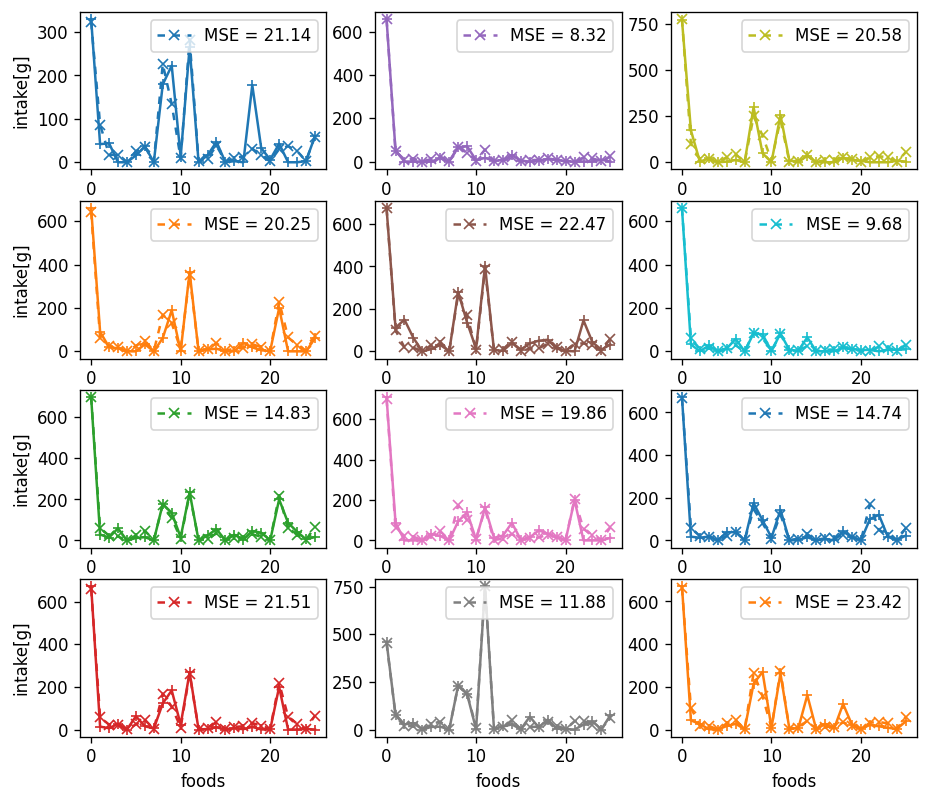| **Figure 7**. Snapshots of original dietary pattern and decoded pattern using Auto Encoder. The loss function is Mean Square Error. The AE learn global(macro) information about food absorbing. It predict major food accurately. But the AE cannot catch micro information about difference. |

The embeded code doesn't show difference between DM and non-DM clearly. In other words, AE learn global information to some extent. But the micro information, which can make remarkable difference in DM prevalence, isn't learned enough.

|  |
| :----------------------------------------------------------: |
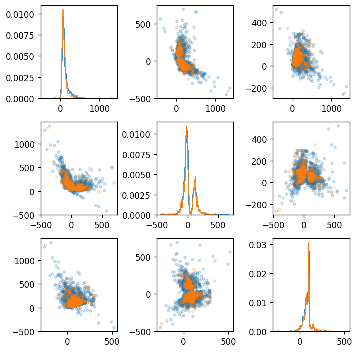| **Figure 8**. Embeded code($dim=3$) obtained by Auto Encoder from dietary pattern. The blue(orange) circle means normal subject(diabetes mellitus). The graphs of diagonal parts is histogram of each embeded dimension. |

## Discussion

- Is this valid to determine a set of micro(?) cluster with different levels (not overlapped)?
- Is this valid statistically?
- Is it possible to train the machine learning model or neural network model?

[^1]: Kim, Y., B.G. Han, and G.E.S.g. Ko, *Cohort Profile: The Korean Genome and Epidemiology Study (KoGES) Consortium.* Int J Epidemiol, 2017. **46**(4): p. 1350.
[^2]: J. E., Lee, et al. "Dietary pattern classifications with nutrient intake and health-risk factors in Korean men." *Nutrition* 27.1 (2011): 26-33.
[^3]: American Diabetes, A., *2. Classification and Diagnosis of Diabetes: Standards of Medical Care in Diabetes-2021.* Diabetes Care, 2021. **44**(Suppl 1): p. S15-S33.
[^4]: Expert Committee on the, D. and M. Classification of Diabetes, *Report of the expert committee on the diagnosis and classification of diabetes mellitus.* Diabetes Care, 2003. **26 Suppl 1**: p. S5-20.
[^5]: American Diabetes, A., *Diagnosis and classification of diabetes mellitus.* Diabetes Care, 2014. **37 Suppl 1**: p. S81-90.
[^6]: Blondel, Vincent D., et al. "Fast unfolding of communities in large networks Journal of Statistical Mechanics: Theory and Experiment 2008." *P10008* (2008).
[^7]: Bonald, Thomas, et al. "Scikit-network: Graph Analysis in Python." *J. Mach. Learn. Res.* 21 (2020): 185-1.

------------------------------------------------

## Supplementary Material

#### Table1. The baseline characteristics for each typical micro cluster

| | High risk group | | | Low risk group | | |
| ------------------------------------- | --------------- | -------------- | --------------- | --------------- | --------------- | --------------- |
| | **C10** | **C11** | **C12** | **C3** | **C13** | **C15** |
| Number of participants (n) | 127 | 118 | 109 | 213 | 107 | 102 |
| NGT, n (%) | 60 (47.2) | 52 (44.1) | 48 (44.0) | 123 (57.7) | 57 (53.3) | 64 (62.7) |
| Prediabetes, n (%) | 67 (52.8) | 66 (55.9) | 61 (56.0) | 90 (42.3) | 50 (46.7) | 38 (37.3) |
| Age, year (mean (sd)) | 54.38 (8.96) | 54.81 (9.31) | 50.71 (8.76) | 50.84 (8.51) | 53.13 (8.66) | 51.26 (8.36) |
| 40~49, n (%) | 47 (37.01) | 41 (34.75) | 63 (57.80) | 101 (47.42) | 37 (34.58) | 48 (47.06) |
| 50~59, n (%) | 30 (23.62) | 26 (22.03) | 17 (15.60) | 45 (21.13) | 32 (29.91) | 22 (21.57) |
| 60~69, n (%) | 40 (31.50) | 40 (33.90) | 23 (21.10) | 39 (18.31) | 25 (23.36) | 21 (20.59) |
| Men, n (%) | 67 (52.76) | 70 (59.32) | 81 (74.31) | 100 (46.95) | 36 (33.64) | 35 (34.31) |
| **Area** | | | | | | |
| Anseong (Rural), n (%) | 68 (53.54) | 73 (61.86) | 61 (55.96) | 111 (52.11) | 77 (71.96) | 52 (50.98) |
| Ansan (Urban), n (%) | 59 (46.46) | 45 (38.14) | 48 (44.04) | 102 (47.89) | 30 (28.04) | 50 (49.02) |
| **Anthropometric measure** | | | | | | |
| Height, cm (mean (sd)) | 159.49 (8.53) | 160.37 (8.52) | 163.28 (8.89) | 160.42 (8.60) | 157.04 (8.39) | 158.29 (7.46) |
| Weight, cm (mean (sd)) | 62.00 (8.60) | 63.29 (9.46) | 64.51 (9.92) | 62.64 (10.04) | 60.79 (9.56) | 62.72 (9.90) |
| BMI, kg/m2 (mean (sd)) | 24.58 (2.82) | 24.36 (2.97) | 24.14 (2.95) | 24.09 (3.01) | 24.59 (2.92) | 25.30 (3.37) |
| Waist circumference, cm | 82.40 (7.97) | 83.09 (8.46) | 82.98 (7.96) | 82.03 (8.59) | 83.32 (8.36) | 82.73 (10.02) |
| Hip circumference, cm (mean (sd)) | 92.71 (5.74) | 92.43 (5.48) | 92.58 (5.83) | 93.18 (5.55) | 93.35 (5.74) | 93.78 (7.13) |
| Waist to Hip Ratio (mean (sd)) | 0.89 (0.07) | 0.90 (0.07) | 0.90 (0.07) | 0.88 (0.08) | 0.89 (0.07) | 0.88 (0.08) |
| **Smoke** | | | | | | |
| Never, n (%) | 74 (58.27) | 60 (50.85) | 36 (33.03) | 122 (57.28) | 73 (68.22) | 73 (71.57) |
| Former, n (%) | 19 (14.96) | 22 (18.64) | 25 (22.94) | 24 (11.27) | 12 (11.21) | 11 (10.78) |
| Current, n (%) | 32 (25.20) | 36 (30.51) | 48 (44.04) | 66 (30.99) | 21 (19.63) | 15 (14.71) |
| **Alcohol** | | | | | | |
| User, n (%) | 5 (3.94) | 13 (11.02) | 10 (9.17) | 13 (6.10) | 3 (2.80) | 9 (8.82) |
| Non-user, n (%) | 55 (43.31) | 43 (36.44) | 27 (24.77) | 95 (44.60) | 59 (55.14) | 61 (59.80) |
| Systolic Blood Pressure, mmHg | 119.24 (18.80) | 119.07 (17.56) | 117.02 (15.92) | 114.75 (18.51) | 117.07 (16.15) | 117.60 (17.46) |
| Diastolic Blood Pressure, mmHg | 75.99 (11.25) | 76.11 (10.45) | 76.55 (10.25) | 73.82 (11.26) | 74.30 (9.70) | 75.60 (11.08) |
| **Laboratory finding** | | | | | | |
| HbA1c, % (mean (sd)) | 5.56 (0.33) | 5.59 (0.41) | 5.56 (0.32) | 5.54 (0.33) | 5.56 (0.35) | 5.51 (0.34) |
| Fasting glucose, mg/dL (mean (sd)) | 84.09 (8.51) | 84.20 (9.36) | 84.38 (9.84) | 81.68 (8.02) | 81.32 (6.93) | 81.25 (7.20) |
| Fasting insulin, µIU/ml (mean (sd)) | 6.95 (4.48) | 6.88 (3.38) | 7.05 (3.88) | 8.06 (5.88) | 8.27 (4.22) | 8.21 (5.19) |
| BUN, mg/dL (mean (sd)) | 14.64 (3.85) | 14.29 (3.37) | 14.37 (3.44) | 14.07 (3.33) | 14.46 (3.98) | 14.17 (3.61) |
| Creatinine, mg/dL (mean (sd)) | 0.84 (0.19) | 0.84 (0.16) | 0.89 (0.17) | 0.84 (0.21) | 0.82 (0.47) | 0.80 (0.15) |
| eGFR, ml/min per 1.73 m2 (mean (sd)) | 90.64 (14.98) | 91.65 (11.90) | 93.18 (14.05) | 93.27 (13.83) | 94.70 (14.61) | 94.19 (13.65) |
| Total cholesterol, mg/dL (mean (sd)) | 188.65 (33.15) | 192.35 (38.00) | 188.39 (36.02) | 185.05 (32.62) | 183.18 (30.48) | 188.44 (36.02) |
| LDL, mg/dL (mean (sd)) | 114.78 (32.01) | 116.97 (33.16) | 105.75 (33.99) | 111.05 (29.71) | 108.55 (29.81) | 114.98 (32.73) |
| HDL, mg/dL (mean (sd)) | 44.98 (10.39) | 43.04 (9.58) | 43.77 (11.23) | 44.52 (10.33) | 44.03 (9.11) | 45.27 (9.26) |
| Triglyceride, mg/dL (mean (sd)) | 144.48 (72.46) | 161.69 (86.93) | 194.37 (124.54) | 149.50 (86.57) | 152.98 (94.01) | 140.94 (60.40) |
| **Insulin resistance index** | | | | | | |
| HOMA-IR (mean (sd)) | 1.44 (0.88) | 1.45 (0.76) | 1.48 (0.80) | 1.63 (1.16) | 1.68 (0.89) | 1.66 (1.08) |
| QUICKI (mean (sd)) | 0.38 (0.05) | 0.38 (0.05) | 0.38 (0.07) | 0.37 (0.06) | 0.37 (0.05) | 0.37 (0.06) |
| **Insulin secretion index** | | | | | | |
| HOMA-β (mean (sd)) | 140.21 (138.12) | 137.41 (89.14) | 146.95 (155.76) | 190.99 (191.80) | 185.21 (119.52) | 182.20 (121.24) |

#### Table2. The baseline characteristics for healthy/critical cluster(lv4) group

| | High risk group (C10+C11+C12) | Low risk group (C3+C13+C15) | p-value | $\chi^2$ |
| ------------------------------------- | --------------------------------- | ------------------------------- | ------- | -------- |
| Number of participants (n) | 354 | 422 | | |
| NGT, n (%) | 160 (45.2) | 244 (57.8) | | |
| Prediabetes, n (%) | 194 (54.8) | 178 (42.2) | | |
| Age, year (mean (sd)) | 53.39 (9.17) | 51.52 (8.55) | 0.003 | 0.03577 |
| 40~49, n (%) | 159 (44.9) | 210 (49.8) | | |
| 50~59, n (%) | 83 (23.4) | 114 (27.0) | | |
| 60~69, n (%) | 112 (31.6) | 98 (23.2) | | |
| Men, n (%) | 218 (61.58) | 171 (40.52) | <0.0001 | |
| **Area** | | | | 0.98444 |
| Anseong (Rural), n (%) | 202 (57.1) | 240 (56.9) | | |
| Ansan (Urban), n (%) | 152 (42.9) | 182 (43.1) | | |
| **Anthropometric measure** | | | | |
| Height, cm (mean (sd)) | 160.95 (8.76) | 159.05 (8.39) | 0.002 | |
| Weight, cm (mean (sd)) | 63.20 (9.34) | 62.19 (9.90) | 0.145 | |
| BMI, kg/m2 (mean (sd)) | 24.37 (2.91) | 24.50 (3.11) | 0.600 | |
| Waist circumference, cm | 82.81 (8.12) | 82.52 (8.90) | 0.647 | |
| Hip circumference, cm (mean (sd)) | 92.58 (5.67) | 93.37 (6.00) | 0.062 | |
| Waist to Hip Ratio (mean (sd)) | 0.89 (0.07) | 0.88 (0.08) | 0.046 | |
| **Smoke** | | | 0.000 | <0.0001 |
| Never, n (%) | 170 (48.02) | 268 (63.51) | <0.0001 | |
| Former, n (%) | 66 (18.64) | 47 (11.14) | <0.0001 | |
| Current, n (%) | 116 (32.77) | 102 (24.17) | <0.0001 | |
| **Alcohol** | | | <0.0001 | 0.038 |
| User, n (%) | 28 (7.91) | 25 (5.92) | <0.0001 | |
| Non-user, n (%) | 125 (35.31) | 215 (50.95) | <0.0001 | |
| Systolic Blood Pressure, mmHg | 118.50 (17.52) | 116.02 (17.69) | 0.051 | |
| Diastolic Blood Pressure, mmHg | 76.20 (10.65) | 74.37 (10.84) | 0.018 | |
| **Laboratory finding** | | | | |
| HbA1c, % (mean (sd)) | 5.57 (0.35) | 5.54 (0.34) | 0.189 | |
| Fasting glucose, mg/dL (mean (sd)) | 84.21 (9.19) | 81.49 (7.55) | <0.0001 | |
| Fasting insulin, µIU/ml (mean (sd)) | 6.96 (3.95) | 8.15 (5.33) | 0.001 | |
| BUN, mg/dL (mean (sd)) | 14.44 (3.56) | 14.19 (3.57) | 0.338 | |
| Creatinine, mg/dL (mean (sd)) | 0.86 (0.17) | 0.82 (0.29) | 0.064 | |
| eGFR, ml/min per 1.73 m2 (mean (sd)) | 91.76 (13.73) | 93.86 (13.97) | 0.036 | |
| Total cholesterol, mg/dL (mean (sd)) | 189.81 (35.65) | 185.40 (32.93) | 0.074 | |
| LDL, mg/dL (mean (sd)) | 112.73 (33.26) | 111.37 (30.50) | 0.553 | |
| HDL, mg/dL (mean (sd)) | 43.96 (10.40) | 44.58 (9.77) | 0.396 | |
| Triglyceride, mg/dL (mean (sd)) | 165.58 (97.70) | 148.31 (83.02) | 0.008 | |
| **Insulin resistance index** | | | | |
| HOMA-IR (mean (sd)) | 1.45 (0.81) | 1.65 (1.07) | 0.006 | |
| QUICKI (mean (sd)) | 0.38 (0.06) | 0.37 (0.06) | 0.081 | |
| **Insulin secretion index** | | | | |
| HOMA-β (mean (sd)) | 141.36 (130.04) | 187.40 (160.20) | <0.0001 | |

#### Figures

|  |
| ------------------------------------------------------------ |
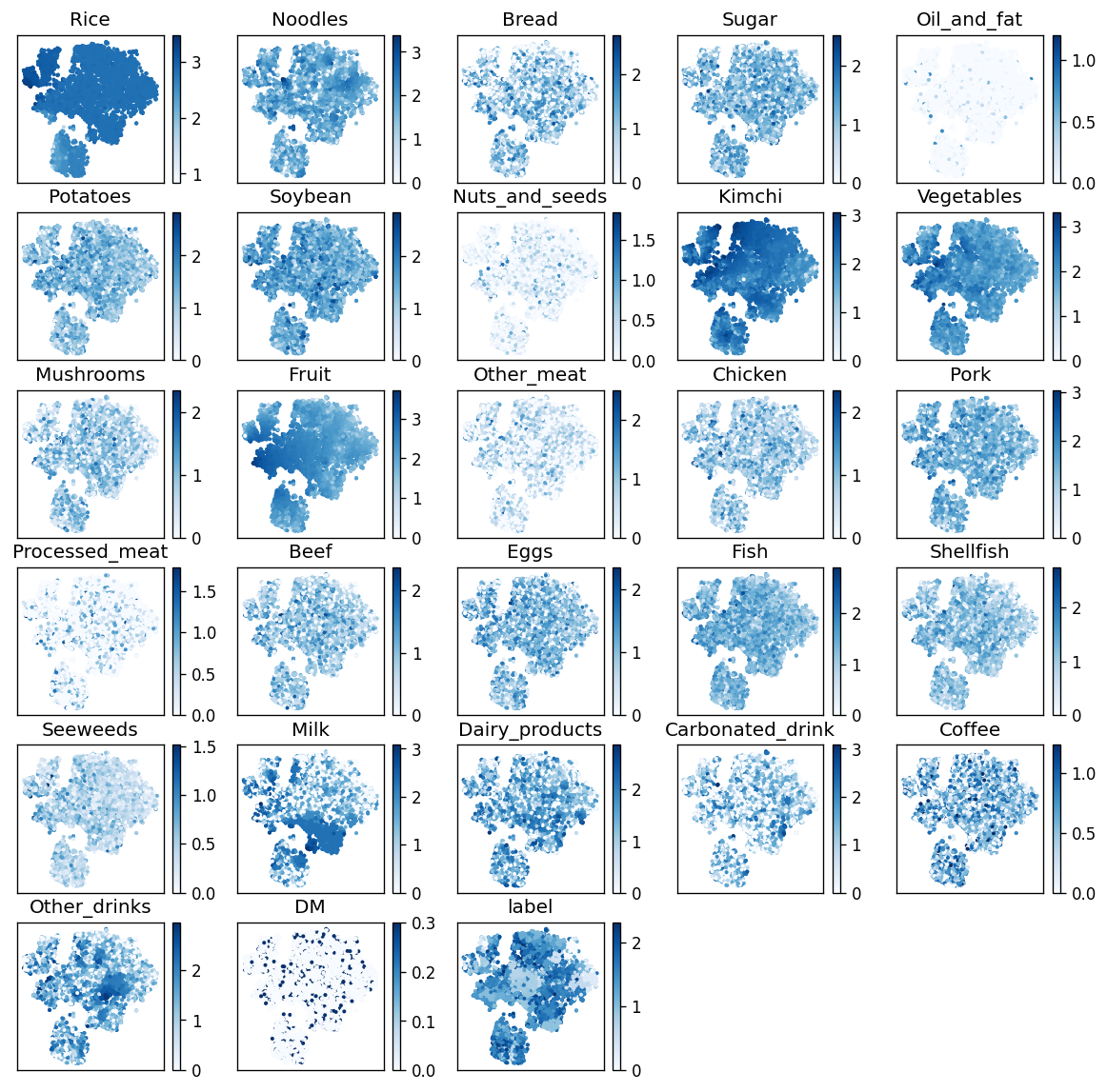| **Figure S1**. Result of manifold learning with t-SNE. The color means logarithmic daily food intake[g], state of Diabetes Mellitus, and the label of clustering(at lv4). Foods with major intake determine the embeding dimension. |

|  |
| :----------------------------------------------------------: |
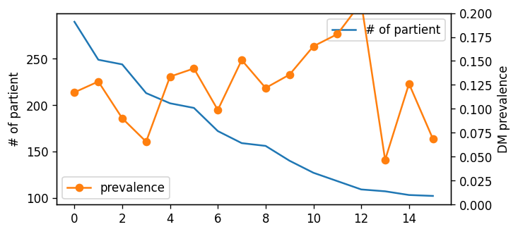| **Figure S2**. Cluster size and its prevalence of typical micro cluster in Lv4. |

|  |
| :----------------------------------------------------------: |
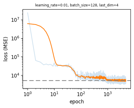| **Figure S3**. Loss function of Auto Encoder. In learning process, there are step-side decreasing regardless of encoded dimension(last dimension). |

|  |
| :----------------------------------------------------------: |
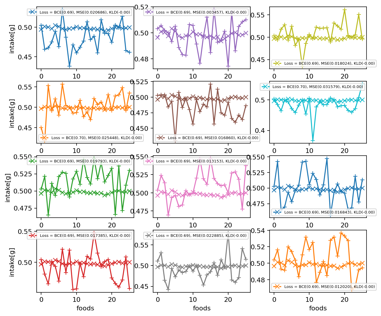| **Figure S4**. Decoded of Variational Auto Encoder. Original dietary pattern(+) and decoded pattern of VAE(x). The VAE doesn't learn just global information. |