# Introduction to parallel programming

## Intro to parallel programming

### 1.1 Welcome to Week 1

Welcome to the course Introduction to parallel programming! I will be your guide through the weeks.
In the first week, we will first introduce the basic principles and paradigms of parallel programming. We will not go deeply into each topic since we will dedicate that to the upcoming weeks, touching even on some advanced topics in parallel programming. We describe the more advanced topics with the purpose of telling you what is important to know and giving you a starting point on where to learn more. We hope that at some point you will be able to do your coding and advance your learning beyond this course.

Many scientific and engineering challenges can be tackled in the area of computing. In general, we have two views on it. One view is distributed serial computing. This means that you have many problems to solve and you don't care about time. The other is parallel computing, where the problem needs to be divided into many compute cores or nodes, essentially many computers because it is too big to fit into one computer or one computer would be too slow to solve it. The first approach is often called grid computing, while the second is generally referred to as supercomputing, where you need a supercomputer to solve your problem. You have probably also heard of cloud computing or similar, which is a commercial version of grid or supercomputing resources.

If you are a serious user, you will quickly learn this. If we use an analogy, buying a car is cheaper than renting it in the long term. There will never be a commercial offering that will match individual purchases for the machine which is usually 90 or 100% utilized. So it's not like buying a car for fun and spending a lot on it. Supercomputers are usually very heavily utilized. This means that during their lifetime, the computer operates near peak performance.

The program is usually written and compiled into instructions for serial execution on one processor (see image below). You have to divide the problem into separate subproblems that can be executed in parallel on many processors available and achieve speedup.


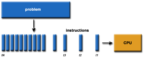
**Source of image: hpc.llnl.gov**

There are different approaches or programming models that were developed during the years and are still being developed. These languages might help you to resolve some of the issues in the underlying hardware topology, that we usually see as a combination of memory and CPUs; both is essential for parallel computing. In the past there was just a single processor per node with memory, and many of those nodes were combined to make a cluster. In recent years a cluster of compute nodes, so-called ["Beowulf"](http://ibiblio.org/pub/Linux/docs/HOWTO/archive/Beowulf-HOWTO.html#ss2.2), is being upgraded with many cores per node and shared memory. The cores share a memory. There can also be many processor sockets, threads per core and GPU accelerators. The programming model for such a hardware architecture is a combination of languages. For example, we have a parallelization called *OpenMP*, that can be easily done on a single computer, whether this is your PC, laptop or a remote computer. OpenMP is quite an easy approach to do "automatic" parallelization. It means that you will start with a serial program and upgrade it with the pragma comment directives. The result is a multi-threaded code that runs faster. We will introduce OpenMP this week, while in Week 2 we will present it in detail.

### 1.2 What team are you on?

We will introduce you to parallel programming with the use of some programming languages.
Please, introduce yourself in the comments area on this page, saying why are you interested in the parallel programming course and what do you hope to gain from it. Are there any specific aspects of the subject that you would like to learn about? Tell us which programming language(s) you use or know about or what language are you planning to learn.

#### About us

The lead educator is Leon Kos, HPC developer/consultant at University of Ljubljana.

The other educators are:

- Matic Brank is an OpenMP consultant at University of Ljubljana
- Leon Bogdanović is a GPU consultant at University of Ljubljana
- Kim Badovinac is a MSc student in Computer Science at University of Ljubljana

Be sure to view their profiles and follow them so you can keep track in the course discussions.

What to expect from us?

We will be monitoring your comments and questions, and try to provide helpful feedback as much as possible. If you find typos or other mistakes, please leave a comment so we can improve the material.

The social aspect of an online course is also very important, so please try to interact with your fellow participants in a constructive way as well.

### 1.3 Interactive notebook use

In this exercise you will learn how to use Jupyter notebooks interactively. All the examples and exercises in this course will be available in such notebooks. We prepared a platform on which you can run notebooks and experiment with them. Alternatively, the notebooks are also available on Google Colaboratory and some of them on Binder.

Click on the *Launch* button below. You will be taken to a page with the Jupyter notebook on our platform. For every exercise in the course you will be directed to a notebook in such a way. In other type of steps, like articles and videos, notebooks will be embedded at the bottom of every step page.

Follow the guide in the notebook to get acquainted with the platform.

You can also repeat the exercise on Google Colaboratory. There are some slight differences in using Jupyter notebooks on Colab. You must create a Google account to run and use them. You should also save copies of the notebooks in Google Drive by `File -> Save a copy in Drive` and then you can run or modify your local copies at will.

[](https://colab.research.google.com/drive/1eHmWppgs9lA7lDuV0afop08qMLgWD2jB)

You can also access the exercise on Binder. Note that the Binder service can take some time to start, but after that you will be able to use all the other notebooks immediately.

[](https://mybinder.org/v2/gh/kosl/ihipp-examples/HEAD?filepath=Interactive_notebook_use_binder.ipynb)

Note also that clicking on the badge "Open in Colab" or "launch binder" will not open a new window or tab in your browser. Therefore you should manually open the link in a new window or tab, if you want to keep the current page in FutureLearn.

**TERMS OF USE**

**The Jupyter notebooks platform on our server can be used solely for the purpose of this course. Any other type of use can result in a connection denial to our server.**

The notebooks require cross-site cookie tracking to be enabled because course exercise pages are composed from two distinct servers. If you experience "Forbidden" or cookie related messages then try a different browser or disable cross-site prevention. For example, in Safari browser choose Safari > Preferences > Privacy and uncheck "Prevent cross-site tracking".

### 1.4 Hello World!

As already mentioned, the simplest approach to parallelization is Open Multi-Processing (OpenMP). We will show you this paradigm through a "Hello World!" example in two programming languages: **C** and **Fortran**.

Let's assume we want to parallelize the "Hello World!" print statement in C:

~~~c
printf("Hello World!\n");
~~~

and in Fortran:

~~~fortran
PRINT *, "Hello World!"
~~~

We can do that with the `parallel` construct which forms a team of threads and starts parallel execution. In C the construct looks like:

~~~c
#pragma omp parallel num_threads(2)
{
printf("Hello World!\n");
}
~~~

Here `#pragma omp` indicates the OpenMP executable directive, `parallel` is the construct and `num_threads(2)` the number of threads to be used. This directive is applied to the succeeding structured block of executable statements between `{...}`. In our case, the executable statement is the "Hello World!" print statement.

In Fortran the construct looks like:

~~~fortran
!$OMP PARALLEL num_threads(2)

PRINT *, "Hello World!"

!$OMP END PARALLEL
~~~

Similarly to C, `!$OMP` indicates the OpenMP executable directive, `PARALLEL` the construct and `num_threads(2)` the number of threads to be used. This directive is applied to the succeeding structured block of executable statements with a single entry at the top and a single exit at the bottom. As before, the executable statement is the "Hello World!" print statement.

First, have a look at the notebook with both the C and Fortran codes. Notice the C headers that must be included and the `USE OMP_LIB` line of code in Fortran to provide OpenMP functionality. We will explain the compilation of the code later, so don't worry about this detail for now.

Run both codes in the notebooks:

[](https://mybinder.org/v2/gh/kosl/ihipp-examples/HEAD?filepath=OpenMP/Hello_world_OpenMP.ipynb)

[](https://colab.research.google.com/drive/1gNK53eCnhFteBtzexMCf5wj7DKvawu2k)

Are the outputs as you expected?

As a bonus example also the OpenMP "Hello World!" in C using [Cling](https://root.cern/cling/) (an interactive C++ interpreter) is given in the notebook below.

### 1.5 Architectures and memory models

Over the years, there have been different multi-node approaches to parallelization. The only really interesting approach is Message Passing Interface (MPI), which we will introduce this week and present in detail in Week 3. Contrary to "automatic" parallelization in OpenMP, we need manual parallelization in MPI.

A combination of both approaches, so called hybrid model with OpenMP and MPI can be also done in a very simple way to gain a bit of performance regarding memory or CPU utilisation (see image below). Latest hardware architectures have non-uniform memory access called NUMA, hence memory regarding the cores is not symmetric but mostly asymmetric.


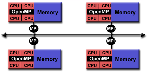
**Source of image: hpc.llnl.gov**

The parallel computing approach tends to use as many computing cores as possible for parallel code execution. The ideal is 100% parallel utilisation, which can be achieved only for embarrassingly simple parallel problems, that is parallel processing of the same subproblems on multiple processors.


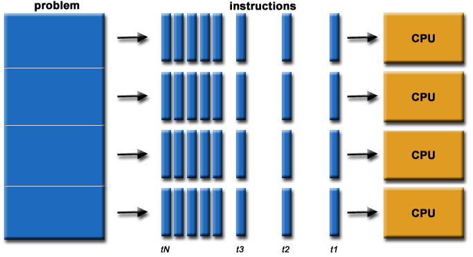
**Source of image: hpc.llnl.gov**

Such kind of computing is actually not considered High Performance Computing (HPC). You have many other solutions, for example, grid computing that is usually distributed or cloud computing that you can rent. Such problems that are being solved are not actually interdependent, so the parallelization here is 100% and no communication is needed among the processes. Running such a problem on HPC would mean the under-utilisation of a supercomputer since the main point of HPC is having closely coupled compute cores on multiple nodes. In such non-dependent cases, you have quite a good scaling, that is, your program can run equally well on one core as on one million cores because there is no interdependence. An example of such embarrassingly simple problems is searching for an optimum of some function for which you do not know its optimum location, so you greedily search the domain.

There can also be some "intelligence" behind using a genetic algorithm, but this actually complicates the problem since there can be an overlap of the search domains. And such algorithms are maybe just empirically describing the theory behind. That's what supercomputing actually is not, although we are very content with such kinds of computing problems. Other problems that can be highly parallel are, for example, some kind of direct numerical computing of fundamental equations or kinetic simulations, which could be very close to how embarrassingly simple computing is.

For efficient parallelization, you need to know the computer architecture on which programs will run. Let's have a look at a computing node found in modern supercomputers. In the picture below, you can observe that the compute node is a standalone "Von Neumann" computer.


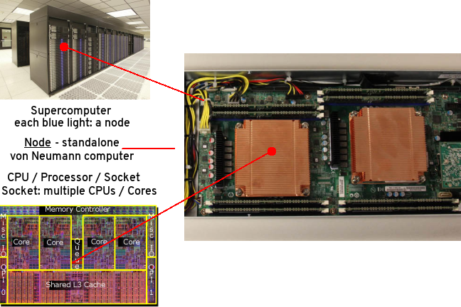
The schematic below shows the logical view of a compute node:


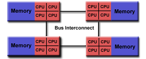
**Source of image: hpc.llnl.gov**

We have two or maybe four CPU sockets with shared memory that are interconnected by a bus or fast bus. The nodes are also connected with fast internet or Infiniband, a network that has small latency. Such architecture was a standard for computers ten years ago. In recent years, mainstream computers besides CPU sockets also have accelerators, that are general-purpose graphical processing units (GPU) for speed up of computing. Therefore, the non-uniform memory is even more non-uniform. Coding or porting old codes with MPI and accelerating parts of it has become increasingly difficult to achieve. We will introduce you to accelerated programming with CUDA and OpenCL in Week 5, that is, how to off-load parts of the code to the accelerators.

Combining everything to run on a large cluster requires quite a lot of experience, with the trial and error approach to identify the bottlenecks. To resolve interconnection problems of nodes in the Infiniband network and among the processor sockets and accelerators (GPUs) in the node, some newer languages or upgrades to the existing programming languages were developed. To utilize these new paradigms, we need to use some new tricks with the old code, although rethinking or rewriting the code is usually the best approach. The new code approaches can be used even without the intervention of a programmer or any thinking, for example, Coarray Fortran has some intelligence behind how to do non-uniform memory operations on matrices and so on, but we actually need to understand a few things.

Let's also discuss how nodes in a supercomputer are interconnected.


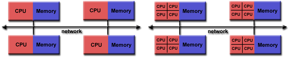
**Source of image: hpc.llnl.gov**

The figure on the left shows the node's architecture which was typical in the past, while the figure on the right shows the current standard: accelerators can also be attached to memory from the other side. Distributed computing in such a sense means that the nodes are interconnected with some kind of topology. The many nodes message exchange, with message passing interface (MPI), is done through a high speed and low latency network, usually using Infiniband or some kind of similar technology, like Tofu interconnect or ARIES, which are actually dependent on the vendor. Infiniband is quite common and a de facto standard among many vendors. That means you can build a cluster with different vendors, which will still work for you, and that was actually the initial idea to use commodity hardware and interconnect it by a high-speed network. This is the basic idea of a supercomputer: a single fast machine that shares memory and processors, which can act well with any code.

A typical test still used to measure the performance of such machines is the [LINPACK test](https://www.top500.org/project/linpack/). Usually, the result is given in TFlops or tera-FLops. 1 TFlops means the capability of a trillion floating-point operations per second. Currently, the [TOP10](https://www.top500.org/lists/top500/2021/11/) supercomputers in the world exceed the 30 thousand TFlops mark with the fastest over 400 thousand TFlops or 400 peta-Flops.

So, for the development of parallel codes, you need to have quite a good overview of the architecture that you are using. Usually, many computing centres provide different machines, depending on the type of users. General-purpose codes are usually not best suited for parallel computing. You need to understand the bottlenecks or which parts of the code consume most of the time. These parts must be optimized, and that is the usual approach for the parallelization of the code.

On HPC, optimal communication is crucial for overcoming the bottlenecks. The main reason for bottlenecks can be generally found in communication among many parts of the code(s). To understand communication, one should generally do a profiling of the codes. Based on the profiling results, one could, for example, distribute the overhead of communication evenly to get rid of its peaks. Of course, this depends on the specific problem. Communication overall is important to be understood, but for embarrassingly simple programs or those that do not have, have little or infrequent communication, any communication network could be just fine, even the plain old ethernet.

On the other hand, for solving large problems with coupled systems of equations, it's important not having large delays among coupled parts. The main difference between plain internet/ethernet and Infiniband is in the latency time or how much time is needed to establish communication from one processor to another and to transfer the data between them, whether the data is small or large. Networks like Infiniband offer low-latency transfer among hardware resources connected to it. If you have such kind of problems with communication, you probably would like to group a bunch of messages into a single message in order to have some useful workload.

We can recap what we said regarding the development of parallel codes with the following points:

- good understanding of the problem being solved in parallel
- identifying how much of the problem can be run in parallel
- bottleneck analysis and profiling give a good picture on scalability of the problem
- optimization and parallelization of parts that consume most of the computing time
- the problem needs to be dissected into parts functionally and logically

### 1.6 Amdahl's and Gustafson's laws explained

When you consider the execution of the code on a number of processors, the speed up achieved with such scaling is typically described by Amdahl's law.


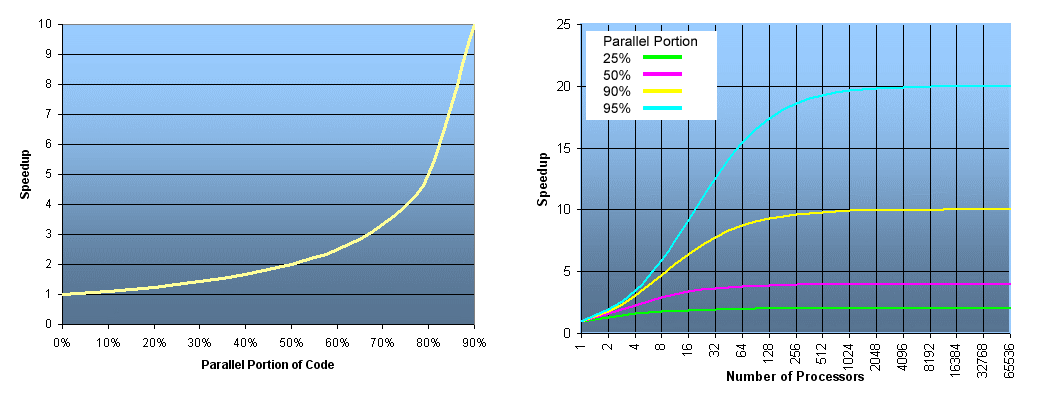
**Source of image: hpc.llnl.gov**

The speed up `S` depends on the parallel portion of the code `p`

$$S = \frac{1}{1-p}$$

The ideal speed up for a code that has, e.g., a parallel portion of 50% or in other words: 50% of it is serial and 50% is parallel, and is executed on an infinite number of processors, is just equal to 2, not more. So, for 50% of the parallel portion of the code, the maximum that you can obtain is two times faster or half of the time that is usually needed for execution on 1 processor (left figure). The figure on the right shows speed up depending on the number of processors for the parallel portion of the code of 25, 50, 90 and 95%, respectively. The mathematical expression for the speed up curves is the following

$$S = \frac{1}{1-p+p/N}$$

where `N` is the number of processors. You can deduce that for a large value of `N` this expression is approximated by the expression given first. For the cyan curve (95% parallel portion of the code), one can observe the maximum speed up of 20x for a large number of processors. A nearly 20x speed up is already achieved with about 500 processors, hence using more than 500 processors will not result in much gain of the speed up.

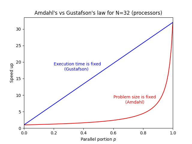
The latter raises the question, why would one invest in one million of processors, if we see that even the best or one of the best programs that are running 95% in parallel, are just going 20x faster? The answer can be given by Gustafson's law that actually interprets the currently available hardware, e.g., if 100, 1000 or a million processors are available to the user.

Such a user can usually tailor the problem to their expectations and the hardware available. In other words, Gustafson's law fixes the time available to the user. By fixing the time, the problem can be scaled to the size that will give you the most accurate result for a chosen run time. Instead of looking at how the code can get faster, one can look for how to get better results in the available run time. For some codes, the expected time for the results to converge can take a week or a month, so we can tailor a problem size to the currently available hardware and get the job done in the specified run time.

The expression for speed up according to Gustafson's law is

$$S = 1 + p(N-1)$$

On the figure below speed up curves according to both laws for `N = 32` are shown. Amdahl's law is often referred to strong scaling, whereas Gustafson's law to weak scaling.


### 1.7 Languages for parallel programming

When speaking of languages for parallel programming, we actually mean parallelization paradigms in host languages. Such paradigms are generally available in the form of Application Programming Interfaces (APIs) that are installed on the user system and can be used as directives or extensions for compiling the parallelized code into executables.

Historically, the first host languages for parallel programming were C/C++ and Fortran. These languages are still a standard for using classical paradigms like OpenMP and MPI and also for accelerated programming, e.g., with CUDA and OpenCL. While Python as an interpreted language is not a common choice for parallel programming, some of its libraries, e.g., Cython, use parallelization paradigms such as OpenMP to speed up Python programs or scripts. A Python library for MPI support exists (mpi4py), although it is not used much in HPC. On the other hand, specialized Python libraries for Machine Learning and Deep Learning in the area of Artificial Intelligence heavily use parallel paradigms for accelerators (GPUs).

In the following list, we give you some parallelization paradigms available as APIs:

* **Open Multi-Processing (OpenMP)**:
- supports multi-platform shared-memory parallel programming in C/C++ and Fortran
- defines a portable, scalable model with a simple and flexible interface for developing parallel applications on several platforms
- annotation of source code to identify the areas that should be accelerated using compiler directives and additional functions
- targets both the CPU and GPU architectures and off-loads computational code on them
* **Message Passing Interface (MPI)**:
- a standardized and portable message-passing standard designed to function on parallel computing architectures
- defines the syntax and semantics of library routines that are useful to a wide range of users writing portable message-passing programs in C, C++, and Fortran.
* **Open Accelerators (OpenACC)**:
- a programming standard for parallel computing designed to simplify parallel programming of heterogeneous CPU/GPU systems
- annotation of C, C++ and Fortran source code to identify the areas that should be accelerated using compiler directives and additional functions
- targets both the CPU and GPU architectures and off-loads computational code on them
* **Compute Unified Device Architecture (CUDA)**:
- a parallel computing platform for general-purpose computing GPUs (GPGPU)
- designed specifically for NVIDIA GPUs
- a software layer for direct access to the GPU's virtual instruction set and parallel computational elements and for the execution of compute kernels
- designed to work with programming languages such as C, C++, and Fortran
* **Open Computing Language (OpenCL)**:
- a framework for writing programs that execute across heterogeneous platforms (CPUs, GPUs, DSPs, FPGAs and other processors or hardware accelerators)
- specifies programming languages (based on C99, C++14 and C++17) for programming these devices to control the platform and execute programs on the compute devices
- provides a standard interface for parallel computing using task-based and data-based parallelism
- an open standard maintained by the non-profit technology consortium Khronos Group
* **SYCL**:
- a higher-level programming model to improve programming productivity on various hardware accelerators
- a single-source domain-specific embedded language (DSEL) based on pure C++17
- a standard developed by Khronos Group
* **Open Hybrid Multicore Parallel Programming (OpenHMPP)**:
- programming standard for heterogeneous computing
- based on a set of compiler directives, a programming model designed to handle hardware accelerators without the complexity associated with GPU programming

### 1.8 Quiz: Intro to parallel programming

This quiz tests your knowledge of basic parallel programming principles and paradigms.

1. What are typical advantages of using parallel codes?

( ) Faster execution than for serial codes

( ) Large amounts of required memory can be distributed

(x) All of the above

Correct.

2. What is a necessary condition for the successful parallelization of the code?

(x) Work can be divided into relatively independent tasks with little communication.

( ) Work can be divided into totally independent tasks with no communication.

Correct.

3. OpenMP is a good choice for code parallelization if (multiple choice answer):

[x] It can be run on a shared memory machine

[ ] It can be run on a distributed memory machine

[ ] The data of the problem can't be partitioned

[x] The data of the problem can be divided into chunks

Correct.

4. What limits the scaling of parallel codes, i.e., their speed up? (multiple choice answer)

[x] Communication bottlenecks

[ ] Memory resources

[x] Synchronization overhead

[x] Serial portion of the code

[ ] Number of processors/cores

Correct.

5. What is the ideal speed up (according to Amdahl's law) for a code that has a parallel portion of 75%?

( ) 2

( ) 3

(x) 4

( ) 5

Correct. For an infinite number of processors the speed up can be calculated by the formula 1/(1-p) or in this case 1/(1-0.75)=4.

## OpenMP overview

### 1.9 Brief intro to OpenMP

OpenMP (Open specifications for Multi Processing) is an API for shared-memory parallel computing. It was developed as an open standard for portable and scalable parallel programming, primarily designed for Fortran and C/C++. It is a flexible and easy to implement solution, which offers a specification for a set of compiler directives, library routines and environment variables.

As of 2021, the latest version of OpenMP API is 5.2. The OpenMP API is comprised of three components:

- Compiler Directives
- Runtime Library Routines
- Environment Variables

Many compilers (proprietary or open source) allow compilation of OpenMP directives in C or Fortran codes. Before using any of them one should [check](https://www.openmp.org/resources/openmp-compilers-tools/) which OpenMP version the compiler's version supports.

**Compiler Directives**

Compiler directives are in the form of comments in the source code and are taken into account at compile time only if an appropriate compiler flag is specified. We use OpenMP compiler directives for:

- spawning a parallel region
- dividing blocks of code among threads
- distributing loop iterations between threads
- serializing sections of code
- synchronization of work among threads

The syntax of the compiler directives is as follows:

sentinel  directive-name  [clause, ...]

In the step Hello World! you have already learned the syntax of the OpenMP compiler directive in C and Fortran, i.e., for the directive name (construct) *parallel*.

**Runtime Library Routines**

These routines can be used for:

* setting and querying:
- number of threads
- dynamic threads feature
- nested parallelism
* querying:
- thread ID
- thread ancestor's identifier
- thread team size
- wall clock time and resolution
- a parallel region and its level
* setting, initializing and terminating:
- locks
- nested locks

All the runtime library routines in C/C++ are subroutines, while in Fortran some are functions, e.g., the runtime library routine for querying the number of threads in C is a subroutine:

~~~c
int omp_get_num_threads(void)
~~~

while in Fortran it is a function:

~~~fortran
INTEGER FUNCTION OMP_GET_NUM_THREADS()
~~~

Also note, that in C/C++ a specific header has to be generally included and that, contrary to Fortran, C/C++ routines are case sensitive:

~~~c
#include <omp.h>
~~~

**Environment Variables**

OpenMP environment variables can be used to control the execution of parallel code at runtime by:

* setting:
- number of threads
- thread stack size
- thread wait policy
- maximum levels of nested parallelism
* specifying how loop interations are divided
* binding threads to processors
* enabling/disabling:
- nested parallelism
- dynamic threads

The OpenMP environment variables are set like any other environment variables, depending on the shell used, e.g., you can set the number of OpenMP threads in *bash* with:

~~~bash
export OMP_NUM_THREADS=2
~~~

and in *csh* with:

~~~bash
setenv OMP_NUM_THREADS 2
~~~

**Compiling codes with OpenMP directives**

You have already seen in the step Hello World! how to compile C and Fortran codes with OpenMP directives:

~~~bash
!gcc hello_world.c -o hello_world -fopenmp
~~~

~~~bash
!gfortran hello_world.f90 -o hello_world.exe -fopenmp
~~~

We used GNU C and Fortran compilers, `gcc` and `gfortran`, respectively, with the compiler flag `-fopenmp` to tell the compiler to take OpenMP directives into account. This flag is dependent on the compiler used, the following table shows which flags have to be used by typical compilers for Unix systems.

| Vendor/Provider | Compiler | Flag |
| :--------------: | :--------------: |:--------------: |
| GNU | `gcc` | `-fopenmp` |
| | `g++` | |
| | `g77` | |
| | `gfortran` | |
| Intel | `icc` | `-openmp` |
| | `icpc` | |
| | `ifort` | |
| PGI | `pgcc` | `-mp` |
| | `pgCC` | |
| | `pgf77` | |
| | `pgf90` | |

### 1.10 OpenMP memory, programming and execution model

OpenMP is based on the shared memory model of multi-processor or multi-core machines. The shared memory type can be either Uniform Memory Access (UMA) or Non-Uniform Memory Access (NUMA). In OpenMP, programs accomplish parallelism exclusively with the use of threads, so called thread-based parallelism.

A thread is the smallest unit of processing that can be scheduled. Threads can exist only within the resources of a single process. When the process is finished, the threads also vanish. The maximum number of threads is equal to the number of processor cores times threads per core available. The actual number of threads used is defined by the user or application used.

In the introduction, we referred to OpenMP as an easy approach for doing "automatic" parallelization. In reality, OpenMP is an explicit *programming model*, which offers the user full control over parallelization. Although not automatic in a strict sense, parallelization is simply achieved by inserting compiler directives in a serial program and hence "automatically" transforming it into a parallel program. Of course, OpenMP also offers complex programming approaches such as inserting subroutines to set multiple levels of parallelism, locks and nested locks, etc.

The basis of OpenMP's *execution model* is the **fork-join model** of parallel execution. OpenMP programs begin as a *master thread* that is executed sequentially until the first parallel region construct is encountered. The master thread then creates a team of parallel threads - a *fork*. The executable statements that are inside the parallel region construct are executed in parallel by the team threads. After the team threads finish execution of the statements in the parallel region construct, synchronization among them occurs and finally their termination results in a *join*, with the master thread as the only thread left.


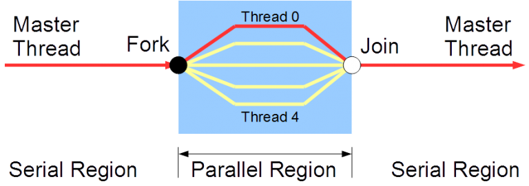
Let's recap the OpenMP terminology discussed so far with descriptions:

| Term | Description |
| :--------------: | :-------------------------------------------: |
| OpenMP thread | a running process specified by OpenMP |
| thread team | a set of threads which cooperate on a task |
| master thread | main thread which coordinates the threads |
| thread safety | specifies correct execution of multiple threads |
| OpenMP directive | OpenMP line of code for compilers with OpenMP |
| construct | an OpenMP executable directive |
| clause | controls the scoping of the variables during execution |

### 1.11 For loop

In this example, you will learn how to use a `for` OpenMP construct (directive-name) in C and a `DO` OpenMP construct (directive-name) in Fortran for vector addition.

Let's assume we want to add arrays `a` and `b` into the sum (array) `c`. In C we can do that by using the `parallel` and `for` OpenMP constructs:

~~~c
#pragma omp parallel shared(a,b,c,chunk) private(i)
{

#pragma omp for schedule(dynamic,chunk) nowait
for (i=1; i <= N; i++)
c[i] = a[i] + b[i];

} /* end of parallel section */
~~~

Let's explain the code in detail:

* in the `parallel` construct:
- the clause `shared(a,b,c,chunk)` indicates that arrays `a`, `b`, `c` and the variable `chunk` will be shared by all threads
- the clause `private(i)` indicates that the variable `i` will be private to each thread and that each thread will have its own unique copy

* in the `for` construct:
- the clause `schedule(dynamic,chunk)` indicates that the iterations of the for loop will be distributed dynamically in `chunk` sizes
- the clause `nowait` indicates that the threads will not synchronize after completing their individual pieces of work

Explore the whole C code in the notebook and run it. Are the results as you expected?

Now, compare the OpenMP code in Fortran with the code in C and identify the differences in the syntax of OpenMP directives (constructs) and clauses.

~~~fortran
!$OMP PARALLEL SHARED(A,B,C,CHUNK) PRIVATE(I)

!$OMP DO SCHEDULE(DYNAMIC,CHUNK)
DO I = 1, N
C(I) = A(I) + B(I)
ENDDO
!$OMP END DO NOWAIT

!$OMP END PARALLEL
~~~

Explore the whole Fortran code in the notebook and run it. Are the results the same as in C?

[](https://mybinder.org/v2/gh/kosl/ihipp-examples/HEAD?filepath=OpenMP/for_DO_OpenMP.ipynb)

[](https://colab.research.google.com/drive/17Db1nJXnuVDKfcPIQtQn8011gkuxyO7n)

### 1.12 Quiz: Intro to OpenMP

This quiz tests your knowledge of the basic principles and programming/execution model of OpenMP.

1. Which of the following about OpenMP is incorrect?

( ) OpenMP is an API that enables explicit multi-threaded parallelism

( ) The primary components of OpenMP are compiler directives, runtime library, and environment variables

( ) OpenMP implementations exist for the Microsoft Windows platform

(x) OpenMP is designed for distributed memory parallel systems and guarantees efficient use of memory

( ) OpenMP supports UMA and NUMA architectures

Correct. OpenMP is not designed for distributed memory parallel systems.

2. OpenMP’s execution model is the *fork-join model* of parallel execution.

(x) True

( ) False

Correct.

3. What statements about the OpenMP execution model are correct? (multiple choice answer)

[x] threads can exist only within the resources of a single process

[ ] threads can exist within the resources of multiple processes

[x] the maximum number of threads is equal to the number of processor cores times threads per core available

[ ] the number of threads to use can't be defined by the user

[ ] a master thread is executed in parallel until the first sequential region construct is encountered

[x] a master thread is executed sequentially until the first parallel region construct is encountered

Correct.

4. Which flag has to be used to tell the `gcc` compiler to take OpenMP directives into account?

( ) `#pragma omp parallel`

( ) `./openmp`

( ) `-openmp`

(x) `-fopenmp`

( ) None of the above

Correct.

5. Which of these is a correct way to set the number of available threads for an OpenMP program to 4?

( ) In an OpenMP program, use the library function `omp_get_num_threads(4)` to set the number of threads to 4 at the beginning of the main function.

( ) In an OpenMP program, use the library function `num_threads(4)` to set the number of threads to 4 at the beginning of the main function.

(x) In bash, `export OMP_NUM_THREADS=4`

( ) In an OpenMP program, use the library function `omp_max_threads(4)` to set the number of threads to 4 at the beginning of the main function.

Correct. All the above library functions can't be used at the beginning of the main function to set the number of available threads.

## MPI overview

### 1.13 Brief intro to MPI

Message Passing Interface (MPI) is a specification of message passing libraries for developers and users. MPI mainly addresses the parallel message-passing programming model. Many open-source MPI implementations exist, which are used for the development of portable and scalable large-scale parallel applications.

The latest released MPI standard is currently MPI 4.0. One should be aware of the version and features of the standard the MPI library implementation at their disposal supports. Many host languages are supported (C/C++, Fortran, Python, Java...). Two of the most used MPI library implementations with the appropriate compilers for Linux systems are presented in the following table.

| MPI library | Language | Compiler |
| :--------------: | :--------------: |:--------------: |
| MVAPICH2 | C | `mpicc` |
| | C++ | `mpicxx` |
| | | `mpic++` |
| | Fortran | `mpif77` |
| | | `mpif90` |
| | | `mpifort` |
| Open MPI | C | `mpicc` |
| | C++ | `mpiCC` |
| | | `mpic++` |
| | | `mpicxx` |
| | Fortran | `mpif77` |
| | | `mpif90` |
| | | `mpifort` |

MPI was originally designed for distributed memory architectures (still a de facto standard for distributed computing), although it also runs today on shared memory or hybrid memory architectures. However, the memory model is inherently a distributed memory model, regardless of the underlying machine's physical architecture. Therefore such a design is suitable for scalability on HPC systems. The programming model is explicit, i.e., the responsibility to correctly identify parallelism and implement parallel algorithms with MPI constructs lies with the user.

The Message-Passing programming paradigm can be described with the following points:

- data is distributed across processors (cores)
- each processor (core) simultaneously performs operations with different data
- processores (cores) may need to interact with each other


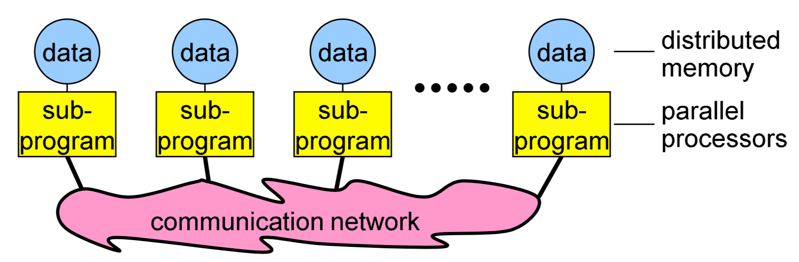
**Image courtesy: Rolf Rabenseifner (HLRS)**

Each processor (core) in an MPI program runs a sub-program, which is typically the same on each processor (core). The variables of each sub-program have the same name but different locations and data (distributed memory), i.e., all variables are private. Processors (cores) communicate via special send and receive routines (message passing).

MPI offers point-to-point as well as collective communications. We will present them in the following step.

### 1.14 Messages and communication

The type of communication in MPI is generally related to the number of processes involved. The simplest form of message passing is *point-to-point communication*, in which one process sends a message to another process. In *collective communication*, several processes are involved at a time. There are 3 classes of such communication: synchronization, data movement and collective computation. Concerning the completion of operations, two types exist: blocking and non-blocking operations. We will briefly describe all the types of communication, you can find details with descriptions of relevant MPI routines in Week 3.

**Messages**

Messages are packets of data moving between sub-programs.


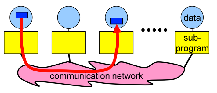
**Image courtesy: Rolf Rabenseifner (HLRS)**

The necessary information for a message-passing system is the following:

- data size and type
- pointer to sent or received data
- sending process and receiving process, i.e., the ranks
- tag of the message
- the communicator, i.e., `MPI_COMM_WORLD`

**Point-to-point communication**

This type relates to communication between two processes. The source process sends a message to the destination process. Processes are identified by their ranks in the communicator.


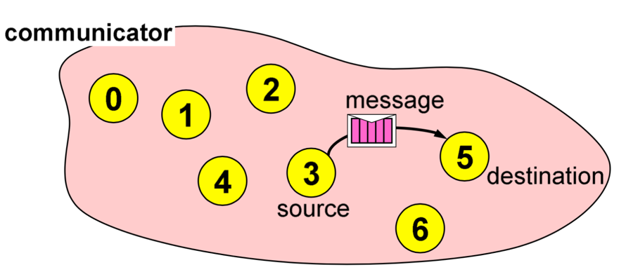
**Image courtesy: Rolf Rabenseifner (HLRS)**

Blocking routines (return only after completion of operations) for send and receive messages:

- `MPI_Send(...)`
- `MPI_Recv(...)`

Non-blocking routines (return immediately and allow sub-programs to perform other work) for send and receive messages:

- `MPI_Isend(...)`
- `MPI_Irecv(...)`

**Collective communication**

Collective operations are of the following type:

- *synchronization*: processes wait until all members of the group have reached the synchronization point
- *data movement*: broadcast, scatter/gather, all to all
- *collective computation* (reductions): one member of the group collects data from the other members and performs an operation (min, max, add, multiply...) on that data

Let's describe some examples of collective communication:

1\. *Broadcast*

Broadcasting can be accomplished by using `MPI_Bcast(...)`. One process sends the same data to all processes in a communicator.
It can be used to send out user input or parameters to all processes. The communication pattern of a broadcast is depicted in the figure below.


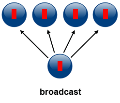
**Source of image: hpc.llnl.gov**

2\. *Scatter*

Scatter can be accomplished by using `MPI_Scatter(...)`. This operation involves a root process sending data to all processes in a communicator. The difference between `MPI_Bcast` and `MPI_Scatter` is the following:

- `MPI_Bcast` sends the same piece of data to all processes
- `MPI_Scatter` sends chunks of data to different processes: after the call the sender has only part of original data available


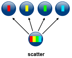
**Source of image: hpc.llnl.gov**

3\. *Gather*

Gather can be accomplished by using `MPI_Gather(...)`. This operation is the inverse of Scatter: it takes elements from many processes and gathers them to one single process.


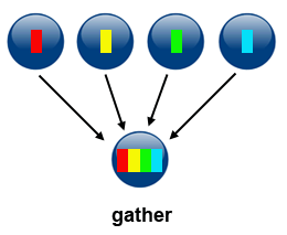
**Source of image: hpc.llnl.gov**

4\. *Reduce*

Reduction can be accomplished by using `MPI_Reduce(...)`. This operation takes an array of input elements on each process and returns an array of output elements to the root process. The output elements contain the reduced result. The image below depicts sum reduction, i.e., an array with four elements of integer type is reduced to an aray with one element containing the sum of the elements of the source array.


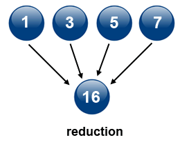
**Source of image: hpc.llnl.gov**

### 1.15 Programming point of view

In this step, we will present how MPI programs are structured, how to compile them and finally, how to run them. The description is pertinent to C/C++, but you can see the differences for other host languages from examples in Week 3.

**MPI program structure**

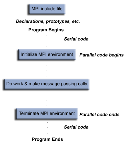
A typical MPI program in C/C++ has the following structure (see figure below):

* inclusion of an MPI header
* declarations of variables and functions, defining prototypes etc.
* main program with:
- serial code
- parallel code: initialization of MPI environment, MPI code (work, calls etc.), termination of MPI environment


An MPI program in C is something like:

~~~c
#include <mpi.h>

int main() {

MPI_Init(NULL,NULL);

MPI_Xxxxxx(parameter, ...);

MPI_Finalize();

return 0;
}
~~~

In this generic example the header file `<mpi.h>` is included. MPI is initialized with `MPI_Init()`, this routine must be called before any other MPI routine. All MPI functions or routines are of the format `MPI_Xxxxxx(parameter, ...)`. MPI is finalized with `MPI_Finalize()`. This routine must be called last by all processes. After it, no further MPI calls may be called.

**Compilation of MPI programs**

Suitable compilers that support MPI or special MPI compilers have to be used for compilation, e.g., one could use

~~~bash
!mpicc hello_world.c -o hello_world
~~~

for compiling MPI codes in C, or:

~~~bash
!mpif90 hello_world.f90 -o hello_world.exe
~~~

for compiling MPI codes in Fortran.

**Running MPI programs**

To run an MPI program `prg` with `num` processes (processors) one should use the following command:

~~~bash
mpirun -np num ./prg
~~~

For example, the executables produced as shown in the previous section can be run with 4 processes (processors) with:

~~~bash
!mpirun -np 4 ./hello_world
~~~

~~~bash
!mpirun -np 4 ./hello_world.exe
~~~

### 1.16 MPI Hello World!

In this exercise, you will be able to run an MPI "Hello World!" example in **C**, **Fortran** and **Python**. This example doesn't make use of any MPI routines, i.e., there is no identification of processes or communication among the processes, so that the compiled code is run on many processors independently with no identification. You will later upgrade this example into an MPI "Hello World!" 2.0 example in which the processes will be identified with the use of MPI calls.

Compare the codes of the different languages in the notebook:

[](https://mybinder.org/v2/gh/kosl/ihipp-examples/HEAD?filepath=MPI/Hello_world_MPI.ipynb)

[](https://colab.research.google.com/drive/1nLztxfsw11_1O-t3622-TxD2b_9C83rK)

How is the MPI library included in the different languages?

Compile and run the codes. Are the results as you expected? Also run the code(s) with the number of processors equal to 128. What is the result?

### 1.17 Quiz: Intro to MPI

This quiz tests your knowledge of the basic principles and programming/execution model of MPI.

1. What is Message Passing Interface (MPI) in principle?

( ) a language for message passing

( ) a library for message passing

(x) a specification a library for message passing

Correct. MPI is in principle a standard or specification for message passing libraries.

2. What statements about point to point communication and collective communication in MPI are correct? (multiple choice answer)

[x] in point to point communication only two processors take part

[ ] in point to point communication many processors can take part

[ ] collective communication can be from one to one, one to many, many to one, or many to many processors

[x] collective communication can be from one to many, many to one, or many to many processors

Correct.

3. In a blocking MPI routine the call returns only after completion of operations.

(x) True

( ) False

Correct. In blocking routines the call returns only after the data is sent out from user buffer to the system buffer in case of `MPI_Send` (or received by the user buffer from the system buffer in case of `MPI_Recv`).

4. What is the difference between `MPI_Bcast` and `MPI_Scatter` routines?

( ) `MPI_Scatter` sends the same piece of data to all processes, `MPI_Bcast` sends chunks of data to different processes

(x) `MPI_Bcast` sends the same piece of data to all processes, `MPI_Scatter` sends chunks of data to different processes

( ) There is no difference, the result of both routines is the same

Correct.

5. What is the correct syntax to run an MPI program `prg` with (on) 4 processes (processors)?

( ) `./prg -np 4`

(x) `mpirun -np 4 ./prg`

( ) `OMP_NUM_THREADS=4 mpirun ./prg`

( ) `OMP_NUM_THREADS=4 ./prg`

Correct. MPI programs are typically run with the `mpirun` command followed by the flag `-np` to specify the number of processes (processors).

## Accelerators overview

### 1.18 Graphics accelerators

Graphics accelerators or graphics processing units (GPUs) are devices with many highly parallel processing units (also called streaming multiprocessors) and very high bandwidth memory. With these two characteristics, they differ from classic processors (CPUs). Apart from their originally intended use, i.e., for intensive 3D graphical rendering (graphics applications), another use is for GPGPU (General Purpose GPU) computing (scientific and engineering applications).

GPUs are more and more used in the area of High-Performance Computing (HPC) because of their much higher power efficiency compared to classic processors (7 clusters out of Top10 on the [Top500 list](https://www.top500.org/lists/top500/list/2021/11/) of supercomputers use GPUs). For example, the fastest most efficient cluster is *Perlmutter*, which is currently #5 on the Top500 list of supercomputers in the world (based on the performance metric in Flops, i.e., floating point operations per second) but is also #7 on the [Green500 list](https://www.top500.org/lists/green500/2021/11/) (based on the power efficiency metric in Flops/watt, i.e., floating point operations per second per watt).

In the context of general-purpose computing, GPUs are referred to as accelerators for intensive computational tasks. The main advantage of GPUs over CPUs is a greater computational capability and high-bandwidth memory, but on the other hand, GPUs are known for latency problems. Thus, efficient computing algorithms make use of the "best of both worlds" approach: GPUs are used for parallel tasks and to achieve throughput performance, while CPUs are used for serial tasks and low-latency access. Therefore, a GPU can be seen as a coprocessor to a CPU, as illustrated in the figure below.


**Source of image: nvidia.com**

Computing acceleration can be achieved with:

- existing GPU applications
- GPU libraries
- directive-based methods (like OpenMP and OpenACC)
- special programming languages or extensions (like CUDA and OpenCL).

### 1.19 GPU Hello World

In this exercise, you will run a GPU "Hello World!" example in **CUDA C** and **PyCUDA**, CUDA extensions to C and Python, respectively. CUDA is a GPU programming extension developed exclusively for NVIDIA GPUs.

Parallel codes that are off-loaded to GPUs are run in so-called kernels. In CUDA C, we define a kernel with the `__global__` prefix, e.g., for the "Hello World!" example we can define the following kernel `hello()`:

~~~c
__global__ void hello()
{
printf("Hello World!\n");
}

~~~

We can call this kernel from the CPU side as a regular function with the triple chevron syntax `<<<...>>>`, e.g.:

~~~c
hello<<<1, 4>>>();
~~~

In this syntax, the first number indicates the number of blocks and the second number the number of threads in a block, i.e., in the above example we defined 1 block with 4 threads to be run in parallel on a GPU.

## Exercise

Run this example in the following notebook.

[](https://colab.research.google.com/drive/1FYIsnTXbvmPcXtZvS2HVimDVSsqSKOE9)

Switch the numbers in the triple chevron syntax, i.e.:

~~~c
hello<<<4, 1>>>()
~~~

and run the example again. Is the result what you expected?

Now, compare the CUDA C code to the equivalent in PyCUDA. Can you identify how the triple chevron syntax in C maps to that in Python?

You have probably noticed that in PyCUDA, the kernel is wrapped as a string of C code; that is what the CUDA implementation in Python actually is: a wrapper of the CUDA C extension.

Note the use of `PATH=/usr/local/cuda-10.1/bin:${PATH}` before the compiler call `nvcc` or the `python` interpreter call: this is needed for older GPUs, e.g., Tesla K80, which are deprecated in the latest versions of CUDA (11.x). Note also that the `pycuda` library must be installed in Python, e.g., through `pip`.

### 1.20 Week 1 wrap-up

In this introductory week we have tried to present you the paradigms of parallel programming by giving the essentials along with simple code examples in interactive Jupyter notebooks. The primary objective of Week 1 is to align you for the next weeks, which you can already preview.

Please discuss the interactive Jupyter notebooks experience and the potentials we are looking forward.
While this week was just a preparation for more advanced topics and hands on examples in the next weeks, we can still discuss how parallel programming techniques could be useful for your applications.

Therefore, we are interested in whether you found the Week 1 content useful?

###### tags:# Introduction to parallel programming

## Intro to parallel programming

### 1.1 Welcome to Week 1

Welcome to the course Introduction to parallel programming! I will be your guide through the weeks.
In the first week, we will first introduce the basic principles and paradigms of parallel programming. We will not go deeply into each topic since we will dedicate that to the upcoming weeks, touching even on some advanced topics in parallel programming. We describe the more advanced topics with the purpose of telling you what is important to know and giving you a starting point on where to learn more. We hope that at some point you will be able to do your coding and advance your learning beyond this course.

Many scientific and engineering challenges can be tackled in the area of computing. In general, we have two views on it. One view is distributed serial computing. This means that you have many problems to solve and you don't care about time. The other is parallel computing, where the problem needs to be divided into many compute cores or nodes, essentially many computers because it is too big to fit into one computer or one computer would be too slow to solve it. The first approach is often called grid computing, while the second is generally referred to as supercomputing, where you need a supercomputer to solve your problem. You have probably also heard of cloud computing or similar, which is a commercial version of grid or supercomputing resources.

If you are a serious user, you will quickly learn this. If we use an analogy, buying a car is cheaper than renting it in the long term. There will never be a commercial offering that will match individual purchases for the machine which is usually 90 or 100% utilized. So it's not like buying a car for fun and spending a lot on it. Supercomputers are usually very heavily utilized. This means that during their lifetime, the computer operates near peak performance.

The program is usually written and compiled into instructions for serial execution on one processor (see image below). You have to divide the problem into separate subproblems that can be executed in parallel on many processors available and achieve speedup.


**Source of image: hpc.llnl.gov**

There are different approaches or programming models that were developed during the years and are still being developed. These languages might help you to resolve some of the issues in the underlying hardware topology, that we usually see as a combination of memory and CPUs; both is essential for parallel computing. In the past there was just a single processor per node with memory, and many of those nodes were combined to make a cluster. In recent years a cluster of compute nodes, so-called ["Beowulf"](http://ibiblio.org/pub/Linux/docs/HOWTO/archive/Beowulf-HOWTO.html#ss2.2), is being upgraded with many cores per node and shared memory. The cores share a memory. There can also be many processor sockets, threads per core and GPU accelerators. The programming model for such a hardware architecture is a combination of languages. For example, we have a parallelization called *OpenMP*, that can be easily done on a single computer, whether this is your PC, laptop or a remote computer. OpenMP is quite an easy approach to do "automatic" parallelization. It means that you will start with a serial program and upgrade it with the pragma comment directives. The result is a multi-threaded code that runs faster. We will introduce OpenMP this week, while in Week 2 we will present it in detail.

### 1.2 What team are you on?

We will introduce you to parallel programming with the use of some programming languages.
Please, introduce yourself in the comments area on this page, saying why are you interested in the parallel programming course and what do you hope to gain from it. Are there any specific aspects of the subject that you would like to learn about? Tell us which programming language(s) you use or know about or what language are you planning to learn.

#### About us

The lead educator is Leon Kos, HPC developer/consultant at University of Ljubljana.

The other educators are:

- Matic Brank is an OpenMP consultant at University of Ljubljana
- Leon Bogdanović is a GPU consultant at University of Ljubljana
- Kim Badovinac is a MSc student in Computer Science at University of Ljubljana

Be sure to view their profiles and follow them so you can keep track in the course discussions.

What to expect from us?

We will be monitoring your comments and questions, and try to provide helpful feedback as much as possible. If you find typos or other mistakes, please leave a comment so we can improve the material.

The social aspect of an online course is also very important, so please try to interact with your fellow participants in a constructive way as well.

### 1.3 Interactive notebook use

In this exercise you will learn how to use Jupyter notebooks interactively. All the examples and exercises in this course will be available in such notebooks. We prepared a platform on which you can run notebooks and experiment with them. Alternatively, the notebooks are also available on Google Colaboratory and some of them on Binder.

Click on the *Launch* button below. You will be taken to a page with the Jupyter notebook on our platform. For every exercise in the course you will be directed to a notebook in such a way. In other type of steps, like articles and videos, notebooks will be embedded at the bottom of every step page.

Follow the guide in the notebook to get acquainted with the platform.

You can also repeat the exercise on Google Colaboratory. There are some slight differences in using Jupyter notebooks on Colab. You must create a Google account to run and use them. You should also save copies of the notebooks in Google Drive by `File -> Save a copy in Drive` and then you can run or modify your local copies at will.

[](https://colab.research.google.com/drive/1eHmWppgs9lA7lDuV0afop08qMLgWD2jB)

You can also access the exercise on Binder. Note that the Binder service can take some time to start, but after that you will be able to use all the other notebooks immediately.

[](https://mybinder.org/v2/gh/kosl/ihipp-examples/HEAD?filepath=Interactive_notebook_use_binder.ipynb)

Note also that clicking on the badge "Open in Colab" or "launch binder" will not open a new window or tab in your browser. Therefore you should manually open the link in a new window or tab, if you want to keep the current page in FutureLearn.

**TERMS OF USE**

**The Jupyter notebooks platform on our server can be used solely for the purpose of this course. Any other type of use can result in a connection denial to our server.**

The notebooks require cross-site cookie tracking to be enabled because course exercise pages are composed from two distinct servers. If you experience "Forbidden" or cookie related messages then try a different browser or disable cross-site prevention. For example, in Safari browser choose Safari > Preferences > Privacy and uncheck "Prevent cross-site tracking".

### 1.4 Hello World!

As already mentioned, the simplest approach to parallelization is Open Multi-Processing (OpenMP). We will show you this paradigm through a "Hello World!" example in two programming languages: **C** and **Fortran**.

Let's assume we want to parallelize the "Hello World!" print statement in C:

~~~c
printf("Hello World!\n");
~~~

and in Fortran:

~~~fortran
PRINT *, "Hello World!"
~~~

We can do that with the `parallel` construct which forms a team of threads and starts parallel execution. In C the construct looks like:

~~~c
#pragma omp parallel num_threads(2)
{
printf("Hello World!\n");
}
~~~

Here `#pragma omp` indicates the OpenMP executable directive, `parallel` is the construct and `num_threads(2)` the number of threads to be used. This directive is applied to the succeeding structured block of executable statements between `{...}`. In our case, the executable statement is the "Hello World!" print statement.

In Fortran the construct looks like:

~~~fortran
!$OMP PARALLEL num_threads(2)

PRINT *, "Hello World!"

!$OMP END PARALLEL
~~~

Similarly to C, `!$OMP` indicates the OpenMP executable directive, `PARALLEL` the construct and `num_threads(2)` the number of threads to be used. This directive is applied to the succeeding structured block of executable statements with a single entry at the top and a single exit at the bottom. As before, the executable statement is the "Hello World!" print statement.

First, have a look at the notebook with both the C and Fortran codes. Notice the C headers that must be included and the `USE OMP_LIB` line of code in Fortran to provide OpenMP functionality. We will explain the compilation of the code later, so don't worry about this detail for now.

Run both codes in the notebooks:

[](https://mybinder.org/v2/gh/kosl/ihipp-examples/HEAD?filepath=OpenMP/Hello_world_OpenMP.ipynb)

[](https://colab.research.google.com/drive/1gNK53eCnhFteBtzexMCf5wj7DKvawu2k)

Are the outputs as you expected?

As a bonus example also the OpenMP "Hello World!" in C using [Cling](https://root.cern/cling/) (an interactive C++ interpreter) is given in the notebook below.

### 1.5 Architectures and memory models

Over the years, there have been different multi-node approaches to parallelization. The only really interesting approach is Message Passing Interface (MPI), which we will introduce this week and present in detail in Week 3. Contrary to "automatic" parallelization in OpenMP, we need manual parallelization in MPI.

A combination of both approaches, so called hybrid model with OpenMP and MPI can be also done in a very simple way to gain a bit of performance regarding memory or CPU utilisation (see image below). Latest hardware architectures have non-uniform memory access called NUMA, hence memory regarding the cores is not symmetric but mostly asymmetric.


**Source of image: hpc.llnl.gov**

The parallel computing approach tends to use as many computing cores as possible for parallel code execution. The ideal is 100% parallel utilisation, which can be achieved only for embarrassingly simple parallel problems, that is parallel processing of the same subproblems on multiple processors.


**Source of image: hpc.llnl.gov**

Such kind of computing is actually not considered High Performance Computing (HPC). You have many other solutions, for example, grid computing that is usually distributed or cloud computing that you can rent. Such problems that are being solved are not actually interdependent, so the parallelization here is 100% and no communication is needed among the processes. Running such a problem on HPC would mean the under-utilisation of a supercomputer since the main point of HPC is having closely coupled compute cores on multiple nodes. In such non-dependent cases, you have quite a good scaling, that is, your program can run equally well on one core as on one million cores because there is no interdependence. An example of such embarrassingly simple problems is searching for an optimum of some function for which you do not know its optimum location, so you greedily search the domain.

There can also be some "intelligence" behind using a genetic algorithm, but this actually complicates the problem since there can be an overlap of the search domains. And such algorithms are maybe just empirically describing the theory behind. That's what supercomputing actually is not, although we are very content with such kinds of computing problems. Other problems that can be highly parallel are, for example, some kind of direct numerical computing of fundamental equations or kinetic simulations, which could be very close to how embarrassingly simple computing is.

For efficient parallelization, you need to know the computer architecture on which programs will run. Let's have a look at a computing node found in modern supercomputers. In the picture below, you can observe that the compute node is a standalone "Von Neumann" computer.


The schematic below shows the logical view of a compute node:


**Source of image: hpc.llnl.gov**

We have two or maybe four CPU sockets with shared memory that are interconnected by a bus or fast bus. The nodes are also connected with fast internet or Infiniband, a network that has small latency. Such architecture was a standard for computers ten years ago. In recent years, mainstream computers besides CPU sockets also have accelerators, that are general-purpose graphical processing units (GPU) for speed up of computing. Therefore, the non-uniform memory is even more non-uniform. Coding or porting old codes with MPI and accelerating parts of it has become increasingly difficult to achieve. We will introduce you to accelerated programming with CUDA and OpenCL in Week 5, that is, how to off-load parts of the code to the accelerators.

Combining everything to run on a large cluster requires quite a lot of experience, with the trial and error approach to identify the bottlenecks. To resolve interconnection problems of nodes in the Infiniband network and among the processor sockets and accelerators (GPUs) in the node, some newer languages or upgrades to the existing programming languages were developed. To utilize these new paradigms, we need to use some new tricks with the old code, although rethinking or rewriting the code is usually the best approach. The new code approaches can be used even without the intervention of a programmer or any thinking, for example, Coarray Fortran has some intelligence behind how to do non-uniform memory operations on matrices and so on, but we actually need to understand a few things.

Let's also discuss how nodes in a supercomputer are interconnected.


**Source of image: hpc.llnl.gov**

The figure on the left shows the node's architecture which was typical in the past, while the figure on the right shows the current standard: accelerators can also be attached to memory from the other side. Distributed computing in such a sense means that the nodes are interconnected with some kind of topology. The many nodes message exchange, with message passing interface (MPI), is done through a high speed and low latency network, usually using Infiniband or some kind of similar technology, like Tofu interconnect or ARIES, which are actually dependent on the vendor. Infiniband is quite common and a de facto standard among many vendors. That means you can build a cluster with different vendors, which will still work for you, and that was actually the initial idea to use commodity hardware and interconnect it by a high-speed network. This is the basic idea of a supercomputer: a single fast machine that shares memory and processors, which can act well with any code.

A typical test still used to measure the performance of such machines is the [LINPACK test](https://www.top500.org/project/linpack/). Usually, the result is given in TFlops or tera-FLops. 1 TFlops means the capability of a trillion floating-point operations per second. Currently, the [TOP10](https://www.top500.org/lists/top500/2021/11/) supercomputers in the world exceed the 30 thousand TFlops mark with the fastest over 400 thousand TFlops or 400 peta-Flops.

So, for the development of parallel codes, you need to have quite a good overview of the architecture that you are using. Usually, many computing centres provide different machines, depending on the type of users. General-purpose codes are usually not best suited for parallel computing. You need to understand the bottlenecks or which parts of the code consume most of the time. These parts must be optimized, and that is the usual approach for the parallelization of the code.

On HPC, optimal communication is crucial for overcoming the bottlenecks. The main reason for bottlenecks can be generally found in communication among many parts of the code(s). To understand communication, one should generally do a profiling of the codes. Based on the profiling results, one could, for example, distribute the overhead of communication evenly to get rid of its peaks. Of course, this depends on the specific problem. Communication overall is important to be understood, but for embarrassingly simple programs or those that do not have, have little or infrequent communication, any communication network could be just fine, even the plain old ethernet.

On the other hand, for solving large problems with coupled systems of equations, it's important not having large delays among coupled parts. The main difference between plain internet/ethernet and Infiniband is in the latency time or how much time is needed to establish communication from one processor to another and to transfer the data between them, whether the data is small or large. Networks like Infiniband offer low-latency transfer among hardware resources connected to it. If you have such kind of problems with communication, you probably would like to group a bunch of messages into a single message in order to have some useful workload.

We can recap what we said regarding the development of parallel codes with the following points:

- good understanding of the problem being solved in parallel
- identifying how much of the problem can be run in parallel
- bottleneck analysis and profiling give a good picture on scalability of the problem
- optimization and parallelization of parts that consume most of the computing time
- the problem needs to be dissected into parts functionally and logically

### 1.6 Amdahl's and Gustafson's laws explained

When you consider the execution of the code on a number of processors, the speed up achieved with such scaling is typically described by Amdahl's law.


**Source of image: hpc.llnl.gov**

The speed up `S` depends on the parallel portion of the code `p`

$$S = \frac{1}{1-p}$$

The ideal speed up for a code that has, e.g., a parallel portion of 50% or in other words: 50% of it is serial and 50% is parallel, and is executed on an infinite number of processors, is just equal to 2, not more. So, for 50% of the parallel portion of the code, the maximum that you can obtain is two times faster or half of the time that is usually needed for execution on 1 processor (left figure). The figure on the right shows speed up depending on the number of processors for the parallel portion of the code of 25, 50, 90 and 95%, respectively. The mathematical expression for the speed up curves is the following

$$S = \frac{1}{1-p+p/N}$$

where `N` is the number of processors. You can deduce that for a large value of `N` this expression is approximated by the expression given first. For the cyan curve (95% parallel portion of the code), one can observe the maximum speed up of 20x for a large number of processors. A nearly 20x speed up is already achieved with about 500 processors, hence using more than 500 processors will not result in much gain of the speed up.

The latter raises the question, why would one invest in one million of processors, if we see that even the best or one of the best programs that are running 95% in parallel, are just going 20x faster? The answer can be given by Gustafson's law that actually interprets the currently available hardware, e.g., if 100, 1000 or a million processors are available to the user.

Such a user can usually tailor the problem to their expectations and the hardware available. In other words, Gustafson's law fixes the time available to the user. By fixing the time, the problem can be scaled to the size that will give you the most accurate result for a chosen run time. Instead of looking at how the code can get faster, one can look for how to get better results in the available run time. For some codes, the expected time for the results to converge can take a week or a month, so we can tailor a problem size to the currently available hardware and get the job done in the specified run time.

The expression for speed up according to Gustafson's law is

$$S = 1 + p(N-1)$$

On the figure below speed up curves according to both laws for `N = 32` are shown. Amdahl's law is often referred to strong scaling, whereas Gustafson's law to weak scaling.


### 1.7 Languages for parallel programming

When speaking of languages for parallel programming, we actually mean parallelization paradigms in host languages. Such paradigms are generally available in the form of Application Programming Interfaces (APIs) that are installed on the user system and can be used as directives or extensions for compiling the parallelized code into executables.

Historically, the first host languages for parallel programming were C/C++ and Fortran. These languages are still a standard for using classical paradigms like OpenMP and MPI and also for accelerated programming, e.g., with CUDA and OpenCL. While Python as an interpreted language is not a common choice for parallel programming, some of its libraries, e.g., Cython, use parallelization paradigms such as OpenMP to speed up Python programs or scripts. A Python library for MPI support exists (mpi4py), although it is not used much in HPC. On the other hand, specialized Python libraries for Machine Learning and Deep Learning in the area of Artificial Intelligence heavily use parallel paradigms for accelerators (GPUs).

In the following list, we give you some parallelization paradigms available as APIs:

* **Open Multi-Processing (OpenMP)**:
- supports multi-platform shared-memory parallel programming in C/C++ and Fortran
- defines a portable, scalable model with a simple and flexible interface for developing parallel applications on several platforms
- annotation of source code to identify the areas that should be accelerated using compiler directives and additional functions
- targets both the CPU and GPU architectures and off-loads computational code on them
* **Message Passing Interface (MPI)**:
- a standardized and portable message-passing standard designed to function on parallel computing architectures
- defines the syntax and semantics of library routines that are useful to a wide range of users writing portable message-passing programs in C, C++, and Fortran.
* **Open Accelerators (OpenACC)**:
- a programming standard for parallel computing designed to simplify parallel programming of heterogeneous CPU/GPU systems
- annotation of C, C++ and Fortran source code to identify the areas that should be accelerated using compiler directives and additional functions
- targets both the CPU and GPU architectures and off-loads computational code on them
* **Compute Unified Device Architecture (CUDA)**:
- a parallel computing platform for general-purpose computing GPUs (GPGPU)
- designed specifically for NVIDIA GPUs
- a software layer for direct access to the GPU's virtual instruction set and parallel computational elements and for the execution of compute kernels
- designed to work with programming languages such as C, C++, and Fortran
* **Open Computing Language (OpenCL)**:
- a framework for writing programs that execute across heterogeneous platforms (CPUs, GPUs, DSPs, FPGAs and other processors or hardware accelerators)
- specifies programming languages (based on C99, C++14 and C++17) for programming these devices to control the platform and execute programs on the compute devices
- provides a standard interface for parallel computing using task-based and data-based parallelism
- an open standard maintained by the non-profit technology consortium Khronos Group
* **SYCL**:
- a higher-level programming model to improve programming productivity on various hardware accelerators
- a single-source domain-specific embedded language (DSEL) based on pure C++17
- a standard developed by Khronos Group
* **Open Hybrid Multicore Parallel Programming (OpenHMPP)**:
- programming standard for heterogeneous computing
- based on a set of compiler directives, a programming model designed to handle hardware accelerators without the complexity associated with GPU programming

### 1.8 Quiz: Intro to parallel programming

This quiz tests your knowledge of basic parallel programming principles and paradigms.

1. What are typical advantages of using parallel codes?

( ) Faster execution than for serial codes

( ) Large amounts of required memory can be distributed

(x) All of the above

Correct.

2. What is a necessary condition for the successful parallelization of the code?

(x) Work can be divided into relatively independent tasks with little communication.

( ) Work can be divided into totally independent tasks with no communication.

Correct.

3. OpenMP is a good choice for code parallelization if (multiple choice answer):

[x] It can be run on a shared memory machine

[ ] It can be run on a distributed memory machine

[ ] The data of the problem can't be partitioned

[x] The data of the problem can be divided into chunks

Correct.

4. What limits the scaling of parallel codes, i.e., their speed up? (multiple choice answer)

[x] Communication bottlenecks

[ ] Memory resources

[x] Synchronization overhead

[x] Serial portion of the code

[ ] Number of processors/cores

Correct.

5. What is the ideal speed up (according to Amdahl's law) for a code that has a parallel portion of 75%?

( ) 2

( ) 3

(x) 4

( ) 5

Correct. For an infinite number of processors the speed up can be calculated by the formula 1/(1-p) or in this case 1/(1-0.75)=4.

## OpenMP overview

### 1.9 Brief intro to OpenMP

OpenMP (Open specifications for Multi Processing) is an API for shared-memory parallel computing. It was developed as an open standard for portable and scalable parallel programming, primarily designed for Fortran and C/C++. It is a flexible and easy to implement solution, which offers a specification for a set of compiler directives, library routines and environment variables.

As of 2021, the latest version of OpenMP API is 5.2. The OpenMP API is comprised of three components:

- Compiler Directives
- Runtime Library Routines
- Environment Variables

Many compilers (proprietary or open source) allow compilation of OpenMP directives in C or Fortran codes. Before using any of them one should [check](https://www.openmp.org/resources/openmp-compilers-tools/) which OpenMP version the compiler's version supports.

**Compiler Directives**

Compiler directives are in the form of comments in the source code and are taken into account at compile time only if an appropriate compiler flag is specified. We use OpenMP compiler directives for:

- spawning a parallel region
- dividing blocks of code among threads
- distributing loop iterations between threads
- serializing sections of code
- synchronization of work among threads

The syntax of the compiler directives is as follows:

sentinel  directive-name  [clause, ...]

In the step Hello World! you have already learned the syntax of the OpenMP compiler directive in C and Fortran, i.e., for the directive name (construct) *parallel*.

**Runtime Library Routines**

These routines can be used for:

* setting and querying:
- number of threads
- dynamic threads feature
- nested parallelism
* querying:
- thread ID
- thread ancestor's identifier
- thread team size
- wall clock time and resolution
- a parallel region and its level
* setting, initializing and terminating:
- locks
- nested locks

All the runtime library routines in C/C++ are subroutines, while in Fortran some are functions, e.g., the runtime library routine for querying the number of threads in C is a subroutine:

~~~c
int omp_get_num_threads(void)
~~~

while in Fortran it is a function:

~~~fortran
INTEGER FUNCTION OMP_GET_NUM_THREADS()
~~~

Also note, that in C/C++ a specific header has to be generally included and that, contrary to Fortran, C/C++ routines are case sensitive:

~~~c
#include <omp.h>
~~~

**Environment Variables**

OpenMP environment variables can be used to control the execution of parallel code at runtime by:

* setting:
- number of threads
- thread stack size
- thread wait policy
- maximum levels of nested parallelism
* specifying how loop interations are divided
* binding threads to processors
* enabling/disabling:
- nested parallelism
- dynamic threads

The OpenMP environment variables are set like any other environment variables, depending on the shell used, e.g., you can set the number of OpenMP threads in *bash* with:

~~~bash
export OMP_NUM_THREADS=2
~~~

and in *csh* with:

~~~bash
setenv OMP_NUM_THREADS 2
~~~

**Compiling codes with OpenMP directives**

You have already seen in the step Hello World! how to compile C and Fortran codes with OpenMP directives:

~~~bash
!gcc hello_world.c -o hello_world -fopenmp
~~~

~~~bash
!gfortran hello_world.f90 -o hello_world.exe -fopenmp
~~~

We used GNU C and Fortran compilers, `gcc` and `gfortran`, respectively, with the compiler flag `-fopenmp` to tell the compiler to take OpenMP directives into account. This flag is dependent on the compiler used, the following table shows which flags have to be used by typical compilers for Unix systems.

| Vendor/Provider | Compiler | Flag |
| :--------------: | :--------------: |:--------------: |
| GNU | `gcc` | `-fopenmp` |
| | `g++` | |
| | `g77` | |
| | `gfortran` | |
| Intel | `icc` | `-openmp` |
| | `icpc` | |
| | `ifort` | |
| PGI | `pgcc` | `-mp` |
| | `pgCC` | |
| | `pgf77` | |
| | `pgf90` | |

### 1.10 OpenMP memory, programming and execution model

OpenMP is based on the shared memory model of multi-processor or multi-core machines. The shared memory type can be either Uniform Memory Access (UMA) or Non-Uniform Memory Access (NUMA). In OpenMP, programs accomplish parallelism exclusively with the use of threads, so called thread-based parallelism.

A thread is the smallest unit of processing that can be scheduled. Threads can exist only within the resources of a single process. When the process is finished, the threads also vanish. The maximum number of threads is equal to the number of processor cores times threads per core available. The actual number of threads used is defined by the user or application used.

In the introduction, we referred to OpenMP as an easy approach for doing "automatic" parallelization. In reality, OpenMP is an explicit *programming model*, which offers the user full control over parallelization. Although not automatic in a strict sense, parallelization is simply achieved by inserting compiler directives in a serial program and hence "automatically" transforming it into a parallel program. Of course, OpenMP also offers complex programming approaches such as inserting subroutines to set multiple levels of parallelism, locks and nested locks, etc.

The basis of OpenMP's *execution model* is the **fork-join model** of parallel execution. OpenMP programs begin as a *master thread* that is executed sequentially until the first parallel region construct is encountered. The master thread then creates a team of parallel threads - a *fork*. The executable statements that are inside the parallel region construct are executed in parallel by the team threads. After the team threads finish execution of the statements in the parallel region construct, synchronization among them occurs and finally their termination results in a *join*, with the master thread as the only thread left.


Let's recap the OpenMP terminology discussed so far with descriptions:

| Term | Description |
| :--------------: | :-------------------------------------------: |
| OpenMP thread | a running process specified by OpenMP |
| thread team | a set of threads which cooperate on a task |
| master thread | main thread which coordinates the threads |
| thread safety | specifies correct execution of multiple threads |
| OpenMP directive | OpenMP line of code for compilers with OpenMP |
| construct | an OpenMP executable directive |
| clause | controls the scoping of the variables during execution |

### 1.11 For loop

In this example, you will learn how to use a `for` OpenMP construct (directive-name) in C and a `DO` OpenMP construct (directive-name) in Fortran for vector addition.

Let's assume we want to add arrays `a` and `b` into the sum (array) `c`. In C we can do that by using the `parallel` and `for` OpenMP constructs:

~~~c
#pragma omp parallel shared(a,b,c,chunk) private(i)
{

#pragma omp for schedule(dynamic,chunk) nowait
for (i=1; i <= N; i++)
c[i] = a[i] + b[i];

} /* end of parallel section */
~~~

Let's explain the code in detail:

* in the `parallel` construct:
- the clause `shared(a,b,c,chunk)` indicates that arrays `a`, `b`, `c` and the variable `chunk` will be shared by all threads
- the clause `private(i)` indicates that the variable `i` will be private to each thread and that each thread will have its own unique copy

* in the `for` construct:
- the clause `schedule(dynamic,chunk)` indicates that the iterations of the for loop will be distributed dynamically in `chunk` sizes
- the clause `nowait` indicates that the threads will not synchronize after completing their individual pieces of work

Explore the whole C code in the notebook and run it. Are the results as you expected?

Now, compare the OpenMP code in Fortran with the code in C and identify the differences in the syntax of OpenMP directives (constructs) and clauses.

~~~fortran
!$OMP PARALLEL SHARED(A,B,C,CHUNK) PRIVATE(I)

!$OMP DO SCHEDULE(DYNAMIC,CHUNK)
DO I = 1, N
C(I) = A(I) + B(I)
ENDDO
!$OMP END DO NOWAIT

!$OMP END PARALLEL
~~~

Explore the whole Fortran code in the notebook and run it. Are the results the same as in C?

[](https://mybinder.org/v2/gh/kosl/ihipp-examples/HEAD?filepath=OpenMP/for_DO_OpenMP.ipynb)

[](https://colab.research.google.com/drive/17Db1nJXnuVDKfcPIQtQn8011gkuxyO7n)

### 1.12 Quiz: Intro to OpenMP

This quiz tests your knowledge of the basic principles and programming/execution model of OpenMP.

1. Which of the following about OpenMP is incorrect?

( ) OpenMP is an API that enables explicit multi-threaded parallelism

( ) The primary components of OpenMP are compiler directives, runtime library, and environment variables

( ) OpenMP implementations exist for the Microsoft Windows platform

(x) OpenMP is designed for distributed memory parallel systems and guarantees efficient use of memory

( ) OpenMP supports UMA and NUMA architectures

Correct. OpenMP is not designed for distributed memory parallel systems.

2. OpenMP’s execution model is the *fork-join model* of parallel execution.

(x) True

( ) False

Correct.

3. What statements about the OpenMP execution model are correct? (multiple choice answer)

[x] threads can exist only within the resources of a single process

[ ] threads can exist within the resources of multiple processes

[x] the maximum number of threads is equal to the number of processor cores times threads per core available

[ ] the number of threads to use can't be defined by the user

[ ] a master thread is executed in parallel until the first sequential region construct is encountered

[x] a master thread is executed sequentially until the first parallel region construct is encountered

Correct.

4. Which flag has to be used to tell the `gcc` compiler to take OpenMP directives into account?

( ) `#pragma omp parallel`

( ) `./openmp`

( ) `-openmp`

(x) `-fopenmp`

( ) None of the above

Correct.

5. Which of these is a correct way to set the number of available threads for an OpenMP program to 4?

( ) In an OpenMP program, use the library function `omp_get_num_threads(4)` to set the number of threads to 4 at the beginning of the main function.

( ) In an OpenMP program, use the library function `num_threads(4)` to set the number of threads to 4 at the beginning of the main function.

(x) In bash, `export OMP_NUM_THREADS=4`

( ) In an OpenMP program, use the library function `omp_max_threads(4)` to set the number of threads to 4 at the beginning of the main function.

Correct. All the above library functions can't be used at the beginning of the main function to set the number of available threads.

## MPI overview

### 1.13 Brief intro to MPI

Message Passing Interface (MPI) is a specification of message passing libraries for developers and users. MPI mainly addresses the parallel message-passing programming model. Many open-source MPI implementations exist, which are used for the development of portable and scalable large-scale parallel applications.

The latest released MPI standard is currently MPI 4.0. One should be aware of the version and features of the standard the MPI library implementation at their disposal supports. Many host languages are supported (C/C++, Fortran, Python, Java...). Two of the most used MPI library implementations with the appropriate compilers for Linux systems are presented in the following table.

| MPI library | Language | Compiler |
| :--------------: | :--------------: |:--------------: |
| MVAPICH2 | C | `mpicc` |
| | C++ | `mpicxx` |
| | | `mpic++` |
| | Fortran | `mpif77` |
| | | `mpif90` |
| | | `mpifort` |
| Open MPI | C | `mpicc` |
| | C++ | `mpiCC` |
| | | `mpic++` |
| | | `mpicxx` |
| | Fortran | `mpif77` |
| | | `mpif90` |
| | | `mpifort` |

MPI was originally designed for distributed memory architectures (still a de facto standard for distributed computing), although it also runs today on shared memory or hybrid memory architectures. However, the memory model is inherently a distributed memory model, regardless of the underlying machine's physical architecture. Therefore such a design is suitable for scalability on HPC systems. The programming model is explicit, i.e., the responsibility to correctly identify parallelism and implement parallel algorithms with MPI constructs lies with the user.

The Message-Passing programming paradigm can be described with the following points:

- data is distributed across processors (cores)
- each processor (core) simultaneously performs operations with different data
- processores (cores) may need to interact with each other


**Image courtesy: Rolf Rabenseifner (HLRS)**

Each processor (core) in an MPI program runs a sub-program, which is typically the same on each processor (core). The variables of each sub-program have the same name but different locations and data (distributed memory), i.e., all variables are private. Processors (cores) communicate via special send and receive routines (message passing).

MPI offers point-to-point as well as collective communications. We will present them in the following step.

### 1.14 Messages and communication

The type of communication in MPI is generally related to the number of processes involved. The simplest form of message passing is *point-to-point communication*, in which one process sends a message to another process. In *collective communication*, several processes are involved at a time. There are 3 classes of such communication: synchronization, data movement and collective computation. Concerning the completion of operations, two types exist: blocking and non-blocking operations. We will briefly describe all the types of communication, you can find details with descriptions of relevant MPI routines in Week 3.

**Messages**

Messages are packets of data moving between sub-programs.


**Image courtesy: Rolf Rabenseifner (HLRS)**

The necessary information for a message-passing system is the following:

- data size and type
- pointer to sent or received data
- sending process and receiving process, i.e., the ranks
- tag of the message
- the communicator, i.e., `MPI_COMM_WORLD`

**Point-to-point communication**

This type relates to communication between two processes. The source process sends a message to the destination process. Processes are identified by their ranks in the communicator.


**Image courtesy: Rolf Rabenseifner (HLRS)**

Blocking routines (return only after completion of operations) for send and receive messages:

- `MPI_Send(...)`
- `MPI_Recv(...)`

Non-blocking routines (return immediately and allow sub-programs to perform other work) for send and receive messages:

- `MPI_Isend(...)`
- `MPI_Irecv(...)`

**Collective communication**

Collective operations are of the following type:

- *synchronization*: processes wait until all members of the group have reached the synchronization point
- *data movement*: broadcast, scatter/gather, all to all
- *collective computation* (reductions): one member of the group collects data from the other members and performs an operation (min, max, add, multiply...) on that data

Let's describe some examples of collective communication:

1\. *Broadcast*

Broadcasting can be accomplished by using `MPI_Bcast(...)`. One process sends the same data to all processes in a communicator.
It can be used to send out user input or parameters to all processes. The communication pattern of a broadcast is depicted in the figure below.


**Source of image: hpc.llnl.gov**

2\. *Scatter*

Scatter can be accomplished by using `MPI_Scatter(...)`. This operation involves a root process sending data to all processes in a communicator. The difference between `MPI_Bcast` and `MPI_Scatter` is the following:

- `MPI_Bcast` sends the same piece of data to all processes
- `MPI_Scatter` sends chunks of data to different processes: after the call the sender has only part of original data available


**Source of image: hpc.llnl.gov**

3\. *Gather*

Gather can be accomplished by using `MPI_Gather(...)`. This operation is the inverse of Scatter: it takes elements from many processes and gathers them to one single process.


**Source of image: hpc.llnl.gov**

4\. *Reduce*

Reduction can be accomplished by using `MPI_Reduce(...)`. This operation takes an array of input elements on each process and returns an array of output elements to the root process. The output elements contain the reduced result. The image below depicts sum reduction, i.e., an array with four elements of integer type is reduced to an aray with one element containing the sum of the elements of the source array.


**Source of image: hpc.llnl.gov**

### 1.15 Programming point of view

In this step, we will present how MPI programs are structured, how to compile them and finally, how to run them. The description is pertinent to C/C++, but you can see the differences for other host languages from examples in Week 3.

**MPI program structure**

A typical MPI program in C/C++ has the following structure (see figure below):

* inclusion of an MPI header
* declarations of variables and functions, defining prototypes etc.
* main program with:
- serial code
- parallel code: initialization of MPI environment, MPI code (work, calls etc.), termination of MPI environment


An MP ipp, HPCFS
The sound and visual effects in the [space waves](https://spacewaves.io) game are very vivid, creating the feeling of flying in space.

Each version of [Moto X3M](https://motox3mgame.org/) —including the original, Winter, Spooky Land, and Pool Party editions—offers new visual themes and hazards, keeping the gameplay fresh for returning players.