淺談主題模型

## <font color = white style="background:rgba(0,0,0,0.6)">淺談主題模型 </font> ### <font color = white style="background:rgba(0,0,0,0.6)">A Brief Introduction to Topic Model</font> ##### <font color = white style = "background:rgba(0,0,0,0.6)">BDSE1211 賴冠州(Ed Lai)</font> --- ## <font color = white style="background:rgba(0,0,0,0.6)">Contents</font> <div style="background:rgba(0,0,0,0.6);margin:auto;width:750px"> <ol> <li>Introduction</li> <li>Latent Dirichlet Allocation (LDA)</li> <li>Variational Algorithms</li>  </ol> </div> --- ## <font color = white style = "background:rgba(0,0,0,0.6)">1. Introduction</font> ----  ## Prerequisites (1/2) - basic calculus, linear algebra - discrete vs. continuous distributions - pmf, pdf, cdf - joint, marginal, conditional distributions - expectation, variance ----  ## Prerequisites (2/2) Bayes Theorem $\boxed{\color{darkorange}{P(H|E)} = \dfrac{\color{green}{P(E|H)}\color{red}{P(H)}}{\color{blue}{P(E)}}}$ - $\color{red}{P(H)}: \text{prior}$ - $\color{green}{P(E|H)}: \text{likelihood}$ - $\color{blue}{P(E)}: \text{marginal evidence}$ - $\color{darkorange}{P(H|E)}: \text{posterior}$ ----  ----  ## What is Data Science? 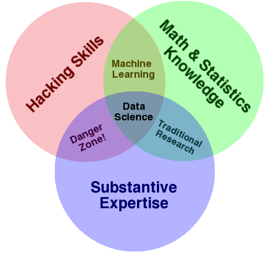(1/2) ![](http://static1.squarespace.com/static/5150aec6e4b0e340ec52710a/t/51525c33e4b0b3e0d10f77ab/1364352052403/Data_Science_VD.png?format=1500w) ----  ## What is Data Science? (2/2) <img src="https://www.predictiveanalyticsworld.com/patimes/wp-content/uploads/2018/05/Medium-Graphic-1.png" alt="aaa" style="max-width:80%;max-height:80%"> ----  ## What is Machine Learning? <img src="https://miro.medium.com/max/1398/1*FUZS9K4JPqzfXDcC83BQTw.png" alt="news" style="width:699px;height:500px"> ----  ## The History of Topic Modeling - Early 90s - LSA (Latent Semantic Analysis) - Analyze relationships between a set of documents and the terms they contain. - tf-idf matrix - Singular value decomposition (SVD) - Late 90s - pLSA (probalistitc LSA) - 2003 - LDA (Latent Dirichlet Allocation) --- ## <font color = white style = "background:rgba(0,0,0,0.6)">2. Latent Dirichlet Allocation</font> ----  ## Model Intuitions (1/3) <img src="https://i.imgur.com/eGrtWQ8.png" alt="news" style="max-width:55%;max-height:55%"> ----  ## Model Intuitions (2/3) ![](https://i.imgur.com/GbgV4Pk.png) ----  ## Model Intuitions (3/3) ![](https://i.imgur.com/N6EUBAe.png) ----  ## Model Assumptions <ol style="font-size:32px"> <li>The order of the words in the document does not matter.</li> <li>The order of documents does not matter.</li> <li>The number of topics is assumed known and fixed.</li> </ol> ----  ## Generative Process (1/3) <div> <ol > <li>Randomly choose a distribution over topics.</li> <li>for each word in the document:</li> <ol style="font-size:36px;list-style-type:lower-latin"> <li>Randomly choose a topic from the distribution over topics in step #1.</li> <li>Randomly choose a word from the corresponding distribution over vocabulary.</li> </ol> </ol> </div> ----  ## Generative Process (2/3) ![](https://i.imgur.com/XCQDCu3.png) $\theta_d \sim \text{Dirichlet}(\alpha)$ $z_{d,n} | \theta_d \sim \text{Categorical}(K, \theta_d)$ $\beta_{k} \sim \text{Dirichlet}(\eta)$ $w_{d,n} | \beta_{1:K}, z_{d,n} \sim \text{Categorical}(K, \beta_k)$ ----  ## Generative Process (3/3) ![](https://i.imgur.com/XCQDCu3.png) $$ \tiny{ \color{brown}{p(\beta_{1:K}, \theta_{1:D}, z_{1:D}, w_{1:D})} = \displaystyle \prod_{k=1}^K p(\beta_k) \displaystyle \prod_{d=1}^D \Bigg( p(\theta_d) \bigg( \displaystyle \prod_{n=1}^N p(z_{d,n} | \theta_d) p(w_{d,n} | \beta_{1:K}, z_{d,n}) \bigg) \Bigg) } $$ ----  ## Bayesian Inference $$ \scriptsize{ \color{darkorange}{p(\beta_{1:K}, \theta_{1:D}, z_{1:D} | w_{1:D})} = \dfrac{\color{green}{p(w_{1:D} | \beta_{1:K}, \theta_{1:D}, z_{1:D})} \color{red}{p(\beta_{1:K}, \theta_{1:D}, z_{1:D})}}{\color{blue}{p(w_{1:D})}} } $$ Two categories of topic modeling algorithms: - Variational algorithms - Sampling-based algorithms --- ## <font color = white style = "background:rgba(0,0,0,0.6)">3. Variational Algorithms</font> ### <font color = white style = "background:rgba(0,0,0,0.6)">Magician's Coin</font> ----  ## Prior and Likelihood (1/8) <ul style="font-size:32px"> <li>The coin belongs to the magician. (prob. may far from 0.5)</li> <li>There’s nothing obviously strange about the coin. (probably a fair coin)</li> </ul> $\color{red}{z} \sim \text{Beta}(\alpha = 3, \beta = 3)$ $\color{green}{x_n|z} \sim \text{Bernouli}(p = z) \quad \forall n = 1, \dots, N$ <img src="https://i.imgur.com/C8qwdVQ.png" > ----  ## Prior and Likelihood (2/8) ```python= z = np.linspace(0, 1, 250) prior_a, prior_b = 3, 3 # prior distribution: Beta[3, 3] p_of_z = scs.beta(prior_a, prior_b).pdf(z) plt.xlabel('z') plt.ylabel('p(z)') plt.plot(z, p_z) plt.show() ``` ----  ## Toss a Coin (3/8) ```python= N = 30 true_prob = scs.uniform.rvs(size = 1) x = scs.bernoulli.rvs(p = true_prob, size = N) print("x =", x) # output: # x = [0 0 0 1 0 0 0 1 0 0 # 0 0 0 0 0 0 0 0 1 0 # 1 1 0 0 0 1 0 0 1 0] ``` ----  ## Posterior (4/8) $\scriptsize{ \color{darkorange}{p(z | \boldsymbol{x})} = \dfrac{ \color{green}{p(\boldsymbol{x} | z)} \color{red}{p(z)} }{ \color{blue}{p(\boldsymbol{x})} } }$ - Find the distribution $\scriptsize{\color{yellow}{q^∗(z)}}$ that is the closest approximation of posterior $\scriptsize{\color{darkorange}{p(z|\boldsymbol{x})}}$. - Let $\scriptsize{\color{yellow}{q(z)} \sim \text{Beta}(\alpha_q, \beta_q)}$ - Measure some sort of distance between two distributions by using $\scriptsize{D_{KL}(Q||P)}$ and our goal is to minimize it. - $\boxed{\tiny{D_{KL}\big( Q(x) || P(x) \big) = \mathbb{E}_{x \sim Q}\big[ \log \frac{Q(x)}{P(x)} \big]}}$ - non-negative but asymmetric. ----  ## Evidence Lower Bound (5/8) $$ \scriptsize{ \begin{aligned} D_{KL}\Big( \color{yellow}{q(z)} \space || \space \color{darkorange}{p(z | \boldsymbol{x})} \Big) &= \mathbb{E}_{\color{yellow}{q}} \big[ \log \frac{\color{yellow}{q(z)}}{\color{darkorange}{p(z | \boldsymbol{x})}}\big] = \mathbb{E}_{\color{yellow}{q}}\Big[ \log \frac{\color{yellow}{q(z)} \color{blue}{p(\boldsymbol{x})}}{\color{green}{p(\boldsymbol{x}|z)} \color{red}{p(z)}} \Big] \\ &= \mathbb{E}_{\color{yellow}{q}}\Big[ \log \color{yellow}{q(z)} \Big] - \mathbb{E}_{\color{yellow}{q}} \Big[ \log \color{green}{p(\boldsymbol{x} | z)} \color{red}{p(z)} \Big] + \mathbb{E}_{\color{yellow}{q}} \Big[ \log \color{blue}{p(\boldsymbol{x})} \Big] \\ &= \mathbb{E}_{\color{yellow}{q}}\Big[ \log \color{yellow}{q(z)} \Big] - \mathbb{E}_{\color{yellow}{q}} \Big[ \log \color{brown}{p(\boldsymbol{x}, z)} \Big] + \log \color{blue}{p(\boldsymbol{x})} \end{aligned} } $$ ----  ## Evidence Lower Bound (6/8) $$ \scriptsize { \begin{aligned} \log \color{blue}{p(\boldsymbol{x})} &= D_{KL}\Big( \color{yellow}{q(z)} \space || \space \color{darkorange}{p(z | \boldsymbol{x})} \Big) - \mathbb{E}_{\color{yellow}{q}}\Big[ \log \color{yellow}{q(z)} \Big] + \mathbb{E}_{\color{yellow}{q}} \Big[ \log \color{brown}{p(\boldsymbol{x}, z)} \Big] \\ &\ge \mathbb{E}_{\color{yellow}{q}} \Big[ \log \color{brown}{p(\boldsymbol{x}, z)} \Big] - \mathbb{E}_{\color{yellow}{q}}\Big[ \log \color{yellow}{q(z)} \Big] = \mathcal{L}(\alpha_q, \beta_q) \end{aligned} } $$ ----  ## Evidence Lower Bound (7/8) $$ \boxed{ \mathcal{L}(\alpha_q, \beta_q) = \mathbb{E}_q \big[ \log p(\boldsymbol{x},z) \big] - \mathbb{E}_q \big[ \log q(z) \big] } $$ - $\scriptsize{\mathcal{L}(\alpha_q, \beta_q)}$ is so called ELBO, evidence lower bound. - Minimizing $\scriptsize{D_{KL}\big(q(z) || p(z|\boldsymbol{x})\big)}$ is equivalent to maximizing $\scriptsize{\mathcal{L}(\alpha_q, \beta_q)}$. ----  ## Evidence Lower Bound (8/8) {%youtube IijEu0_kLcA %} --- ## <font color = white style = "background:rgba(0,0,0,0.6)">References</font> {%pdf https://ai.stanford.edu/~ang/papers/jair03-lda.pdf %} ---- ## <font color = white style = "background:rgba(0,0,0,0.6)">References</font> <div style="background:rgba(0,0,0,0.6);margin:auto;width:1050px"> <ol> <li><a href="https://www.eecis.udel.edu/~shatkay/Course/papers/UIntrotoTopicModelsBlei2011-5.pdf">Introduction to Probabilistic Topic Models</a></li> <li><a href="https://taweihuang.hpd.io/2019/01/10/topic-modeling-lda/">生成模型與文字探勘：利用 LDA 建立文件主題模型</a></li> <li><a href="http://www.openias.org/variational-coin-toss">Variational Coin Toss</a></li> <li><a href="https://medium.com/@tengyuanchang/直觀理解lda-latent-dirichlet-allocation-與文件主題模型-ab4f26c27184">直觀理解 LDA 與文件主題模型</a></li> </ol> </div> ---- ## <font color = white style = "background:rgba(0,0,0,0.6)">References</font> {%youtube ogdv_6dbvVQ %} ---- ## <font color = white style = "background:rgba(0,0,0,0.6)">References</font> <div style="background:rgba(0,0,0,0.6);margin:auto;width:750"> <ol> <li><a href="https://cran.r-project.org/web/packages/lda/index.html"><code style="background-color: gray">lda</code></a> (R package)</li> <li><a href="https://scikit-learn.org/stable/modules/generated/sklearn.decomposition.LatentDirichletAllocation.html"><code style="background-color: gray">sklearn</code></a> (Python package)</li> <li><a href="https://radimrehurek.com/gensim/models/ldamodel.html"><code style="background-color: gray">gensim</code></a> (Python package)</li> <li><a href="https://spark.apache.org/docs/2.3.4/mllib-clustering.html#latent-dirichlet-allocation-lda"><code style="background-color: gray">PySpark</code></a> (Python package)</li> </ol> </div> --- ## <font color = white style = "background:rgba(0,0,0,0.6)">The End</font>