# Some Methods for Working with Probabilistic Models in Machine Learning

One humorous saying that I really like is: ***"Because I’m certain that in this world, nothing is certain..."***.

You are living in an era of ***constant change***; in other words, many things in life always carry a degree of uncertainty.

This is also closely related to many problems in machine learning:
+ Whether the chosen model is suitable for the data. ***This itself is uncertain***. It can be great to use ***linear models*** to approximate ***linear data***, but it would be terrible to use a ***linear model*** to approximate ***nonlinear data***.

+ Whether the collected data is reliable and trustworthy.

+ For some models, we must ***make certain assumptions***. This is also a form of uncertainty.

Instead of deliberately ***avoiding*** it, why not face the truth?

As we all know, when talking about ***uncertainty***, we cannot avoid mentioning a famous field: ***probability theory***, with its many ***interesting theories***.

Applying probability theory to machine learning has given rise to ***probabilistic models***.

As you know, when talking about ***probability theory***, we must talk about ***probability distributions***. For each ***probability distribution***, we have a ***probability mass function for discrete variables*** and a ***probability density function for continuous variables***, and these ***functions*** have parameters. In the article ***[Statistical Samples and the Problem of Estimation in Probability]()***, I denoted these parameters by $\theta$.

Our task now is to ***learn the best probabilistic model for a given dataset***. That is: ***you need to estimate the parameter $\theta$*** so that ***the probabilistic model fits the data as well as possible***.

If you have read my article ***[Statistical Samples and the Problem of Estimation in Probability]()***, then you already know a method of ***point estimation*** for these parameters. This method aims to ***estimate parameters such that the probability of observing the sample points is maximized***. In machine learning, this method is called ***MLE***. In this article, I will also mention some other methods.

## 1. Probabilistic Models

As we know, for some models we often make certain ***(assumptions)***. For example, linear models assume that the data we are working with can be approximated by some linear function.

Probabilistic models are no different. We assume that the data follows certain distributions ***(Bernoulli distribution, Gaussian distribution, Poisson distribution, ...)***, or we make assumptions about the data generation process.

***In probabilistic models, there are different types of variables, and each type has its own characteristics:***

+ **Observed variables** are variables that describe what we can observe ***(e.g., movie ratings, number of views of a movie, ...)***.

+ **Hidden variables** are variables that describe hidden attributes of the data that we cannot directly collect ***(e.g., whether a movie carries strong humanistic values, whether the movie is truly attractive, ...)***.

In probabilistic models, we make assumptions that ***variables*** follow certain distributions. A probabilistic model can have many variables, which also means it can have many assumptions.

In addition to variables, when we place assumptions on parameters ***(e.g., parameters of a probability mass function or probability density function)***, we call such a model a ***Bayesian*** model.

***Here is an example:***

Suppose I have a dataset of students’ exam scores, specifically ***the number of students at each score level*** for the courses ***Introduction to Machine Learning and Data Mining*** and ***Data Science*** at university ***X***, as shown below:


You can view the full dataset ***[here]()***.

I assume that ***the ML & DM scores follow a Gaussian distribution***, ***the Data Science scores follow a Gaussian distribution***, and ***the combined scores of both courses follow a Gaussian distribution***.

***As in the previous article***, I presented a method for ***point estimation of parameters***, with a specific example for the ***Gaussian distribution***.

***The estimators for the parameters of the Gaussian distribution are:***

+ $\hat{\alpha} = \bar{X} = \frac{1}{n}\sum\limits_{i=1}^n x_i$
+ $\hat{\sigma}^2 = S^2 = \frac{1}{n}\sum\limits_{i=1}^n (x_i - \bar{X})^2$

These are exactly the values that make the probability density function fit the data best.

We compute these values separately for ***ML & DM***, ***Data Science***, and for the entire dataset.

We obtain:

+ ***ML & DM:*** $\hat{\alpha} = 5.78, \hat{\sigma} = 1.29$
+ ***Data Science:*** $\hat{\alpha} = 7.07, \hat{\sigma} = 1.26$
+ ***Both courses:*** $\hat{\alpha} = 6.46, \hat{\sigma} = 1.43$

From these values, we obtain the probabilistic models that best fit the data.


+ The blue curve is the best-fitting model for the ***ML & DM*** course. In other words, the blue curve is the Gaussian distribution learned from the ***ML & DM*** data.

+ The red curve is the Gaussian distribution learned to best fit the ***Data Science*** data.

+ The purple curve is the Gaussian distribution learned to best fit the entire dataset (***both courses***).

***The problem is:*** If we use only one of the three models, we cannot correctly describe the entire dataset. In particular, ***the purple curve cannot correctly describe both courses***.

***The reason the purple curve fails*** is that it tries to force the score data of both courses into a single Gaussian distribution, whereas each course actually follows a different Gaussian distribution. Therefore, we cannot use ***a single Gaussian distribution*** to approximate the entire dataset.

At this point, we arrive at the ***GMM – Gaussian Mixture Model***.

***Assume*** that our data is generated from $k$ Gaussian distributions, and each data point is generated from only one of these $k$ distributions. Assume that each data point $x$ has only one attribute.

We then have $k$ sets of parameters $\{ (\mu_1, \sigma_1), (\mu_2, \sigma_2), (\mu_3, \sigma_3), ..., (\mu_k, \sigma_k) \}$ corresponding to the $k$ Gaussian distributions.

Let $Z$ be a variable that follows a multinomial distribution, whose value indicates the index of the distribution chosen when randomly selecting one of the $k$ distributions. The possible values of $Z$ are: $[1, 2, 3, ..., k]$.

The probability mass function of $z$ is:

\begin{equation}
p(z = i) = p_i
\end{equation}

where $p_i$ is the probability that a randomly chosen data point is generated by the $i$-th distribution.
***$p = [p_1, p_2, ..., p_k],\; p_i \ge 0$ are the parameters of the multinomial distribution satisfying $p_1 + p_2 + \dots + p_k = 1$.***

For ***our example above***, the set of possible values of $Z$ is $[1, 2]$.
That is, $P(z = 1 \mid p) = p_1 = 1 - P(z = 2 \mid p)$.

***The density function of the GMM is as follows:***

\begin{equation}
p_1 f(x \mid \mu_1, \sigma_1^2) + p_2 f(x \mid \mu_2, \sigma_2^2) + \dots + p_k f(x \mid \mu_k, \sigma_k^2)
\end{equation}

***Where: $f(x \mid \mu_i, \sigma_i^2)$ is the familiar Gaussian density function:***

\begin{equation}
f(x \mid \mu_i, \sigma_i^2) = \frac{1}{\sigma_i \sqrt{2\pi}} e^{-\frac{(x - \mu_i)^2}{2 \sigma_i^2}}
\end{equation}

If each variable $x$ has multiple dimensions, then the ***GMM*** method is called a ***multivariate GMM***. In this case, the density function of the ***GMM*** is:

\begin{equation}
p_1 f(x \mid \mu_1, \Sigma_1) + p_2 f(x \mid \mu_2, \Sigma_2) + \dots + p_k f(x \mid \mu_k, \Sigma_k)
\end{equation}

***Where: $f(x \mid \mu_i, \Sigma_i)$ is the Gaussian density function for a multivariate variable $x$:***

\begin{equation}
f(x \mid \mu_i, \Sigma_i) = \frac{1}{\sqrt{det(2\pi \Sigma_i)}} e^{-\frac{1}{2}(x - \mu_i)^T \Sigma_i^{-1}(x - \mu_i)}
\end{equation}

The two models introduced above can be used to solve ***classification problems***.

Training, therefore, means learning the parameters.

For a ***multivariate GMM***, we need to learn $k$ sets of parameters
$\{ (\mu_1, \Sigma_1), (\mu_2, \Sigma_2), \dots, (\mu_k, \Sigma_k) \}$
and the parameter vector $p = [p_1, p_2, \dots, p_k]$.

***To learn how to estimate these parameters, please continue to the next section.***

## 2. The MLE Method

You should read the article ***[Statistical Samples and the Problem of Estimation in Probability]()*** before learning about ***MLE***, because the idea behind ***MLE*** is about 99.99% similar to point estimation.

Point estimation requires us to know a dataset $x_1, x_2, \dots, x_n$ sampled from a population ***(e.g., height data of 100 Asian people)***. Given this known dataset, the ***MLE*** method uses the ***training set***.

The point estimation method in the article ***[Statistical Samples and the Problem of Estimation in Probability]()*** seeks the parameter set $\theta$ such that the function $L(x \mid \theta)$ achieves the maximum possible value.

Assume the underlying random variable $X$ has a probability mass function or density function $f(x \mid \theta)$.

\begin{equation}
P(x \mid \theta) = P(X_1 = x_1, X_2 = x_2, \dots, X_n = x_n \mid \theta) = \prod_{i=1}^n f(x_i \mid \theta)
\end{equation}

\begin{equation}
\hat{\theta} = \arg\max_{\theta} \prod_{i=1}^n f(x_i \mid \theta)
\end{equation}

The function $P(x \mid \theta)$ is also called the ***likelihood function***.

This expression holds because the variables in the dataset are ***independent*** of each other. The ***MLE*** method also assumes that the ***$n$ data points*** are independent.

The function $f(x_i \mid \theta)$ in ***MLE*** is precisely the probability distribution.

We can summarize the MLE method as follows:
+ MLE assumes that data points are independent.
+ The point estimates for the parameters of the ***probability mass function*** or ***density function*** in the article ***[Statistical Samples and the Problem of Estimation in Probability]()*** are exactly the optimal parameter values that ***MLE*** needs to learn.

Examples:

+ The best point estimate for the parameter $\lambda$ of the ***Poisson*** distribution is
$\hat{\lambda} = \frac{\sum_{i=1}^n x_i}{n}$, which is also the optimal parameter value learned by ***MLE*** from the ***training*** data.

+ The point estimates for the parameters of the Gaussian distribution (one-dimensional data):
+ $\hat{\alpha} = \bar{X} = \frac{1}{n} \sum_{i=1}^n x_i$
+ $\hat{\sigma}^2 = S^2 = \frac{1}{n} \sum_{i=1}^n (x_i - \bar{X})^2$

These are exactly the values that ***MLE*** needs to learn.

***Difficulties of the MLE method:***

+ Complex data and complex density functions
+ High computational cost for derivative calculations

For example, in the ***multivariate Gaussian*** model:

+ $\mu = [\mu_1, \mu_2, \dots, \mu_k]$
+ $\Sigma = [\Sigma_1, \Sigma_2, \dots, \Sigma_k]$
+ $p = [p_1, p_2, \dots, p_k]$

Assume the data samples $x$ are independent. According to ***MLE***, we need to maximize the following function:

\begin{equation}
\log(P(x_1, x_2, \dots, x_n \mid \mu, \Sigma, p))
= \sum_{i=1}^n \log(P(x_i \mid \mu, \Sigma, p))
= \sum_{i=1}^n \log \sum_{j=1}^k p_j f(x_i \mid \mu_j, \Sigma_j)
\end{equation}

Where:

\begin{equation}
f(x_i \mid \mu_j, \Sigma_j) = \frac{1}{\sqrt{det(2\pi \Sigma_j)}}
e^{-\frac{1}{2}(x_i - \mu_j)^T \Sigma_j^{-1}(x_i - \mu_j)}
\end{equation}

The function $\log(P(x_1, x_2, \dots, x_n \mid \mu, \Sigma, p))$ is very complex.

To reduce the complexity of the model, I would like to introduce a method called ***EM***.

## 3. The EM Method – Expectation Maximization

### 3.1 Explaining the Nature of the Algorithm

Let $Z$ be a variable that follows a multinomial distribution whose value indicates the index of the distribution when randomly selecting one of the $k$ distributions. The possible values of $Z$ are:
$[1, 2, 3, ..., k]$.

Let:
+ $\theta$ be the set of parameters $(\mu, \Sigma, p)$
+ The dataset be $D = (x_1, x_2, ..., x_n)$

That is,
$$
\log(P(x_1, x_2, ..., x_n \mid \mu, \Sigma, p)) = \log(P(D \mid \theta))
$$

As we know, the function $P(D \mid \theta)$ is the probability of observing the dataset $D$.

Instead of directly maximizing $\log(P(D \mid \theta))$, the $EM$ method searches for a ***less complex lower bound*** and ***maximizes that lower bound***.

Specifically, we seek a function $h(\theta)$ such that:
$$
\log(P(D \mid \theta)) \ge h(\theta)
$$
and then solve the optimization problem for $h(\theta)$.

Each data point can belong to only one of the $k$ Gaussian distributions. In other words, the events $Z = 1, Z = 2, ..., Z = k$ form a ***complete set***.

We have:
$$
\log(P(x \mid \theta)) = \log \sum_{i=1}^k P(Z = i, x \mid \theta)
$$

By ***Bayes’ rule***, we have:
$$
P(Z = i, x, \theta) = P(Z = i, x \mid \theta) P(\theta)
$$

$$
P(Z = i, x, \theta) = P(Z = i \mid x, \theta) P(x, \theta)
= P(Z = i \mid x, \theta) P(x \mid \theta) P(\theta)
$$

Thus:
$$
P(Z = i, x \mid \theta) = P(Z = i \mid x, \theta) P(x \mid \theta)
$$

Hence:
$$
\log(P(x \mid \theta))
= \log \sum_{i=1}^k P(Z = i \mid x, \theta) P(x \mid \theta)
= \log E_{Z \mid x, \theta}[P(x \mid \theta)]
$$

To reduce the complexity of the above expression:

***We consider the following auxiliary problem:***

$$
\log E[X] \ge E[\log(X)]
$$

where:
$$
X \text{ takes only non-negative values}
$$

***Proof:***

We have:
$$
n \times \log E[X] = n \times \log\left(\frac{x_1 + x_2 + ... + x_n}{n}\right)
$$

$$
n \times E[\log(X)] = \log(x_1) + \log(x_2) + ... + \log(x_n)
$$

Thus, the auxiliary problem is equivalent to:
$$
\log\left(\frac{x_1 + x_2 + ... + x_n}{n}\right)^n
\ge \log(x_1) + \log(x_2) + ... + \log(x_n)
$$

$$
\iff
$$

$$
\left(\frac{x_1 + x_2 + ... + x_n}{n}\right)^n
\ge e^{\log(x_1) + \log(x_2) + ... + \log(x_n)}
$$

$$
\iff
$$

$$
\left(\frac{x_1 + x_2 + ... + x_n}{n}\right)^n
\ge x_1 x_2 ... x_n
$$

***By the Cauchy inequality:***

For positive numbers $x_1, x_2, ..., x_n$:
$$
x_1 + x_2 + ... + x_n \ge n \sqrt[n]{x_1 x_2 ... x_n}
$$

$$
\Rightarrow \left(\frac{x_1 + x_2 + ... + x_n}{n}\right)^n
\ge x_1 x_2 ... x_n
$$

Thus, ***the auxiliary problem is proven***.

Applying this result to the original problem, we obtain:
$$
\log(P(x \mid \theta))
= \log E_{Z \mid x, \theta}[P(x \mid \theta)]
\ge E_{Z \mid x, \theta}[\log(P(x \mid \theta))]
= \sum_{i=1}^k P(Z = i \mid x, \theta) \log P(x \mid \theta)
$$

Therefore, ***a lower bound of $\log(P(D \mid \theta))$*** is:
$$
\sum_{i=1}^k P(Z = i \mid D, \theta) \log P(D \mid \theta)
$$

Applying this to the entire dataset $D$, assuming the $n$ data points are independent:

\begin{equation}
\log(P(D \mid \theta))
= \sum_{j=1}^n \log(P(x_j \mid \theta))
\ge \sum_{j=1}^n \sum_{i=1}^k P(Z = i \mid x_j, \theta) \log P(x_j \mid \theta)
\end{equation}

We can construct the ***GMM*** model using an idea similar to the ***K-means*** algorithm:

| | K-means | GMM |
| -------- | -------- | -------- |
| Prerequisite | Number of clusters $k$ is predefined | Number of Gaussian distributions is predefined |
| Parameters to learn | $k$ cluster centers | $\mu = [\mu_1, \mu_2, ..., \mu_k]$, $\Sigma = [\Sigma_1, \Sigma_2, ..., \Sigma_k]$, $p = [p_1, p_2, ..., p_k]$ |
| Learning process for each data point $x$ | Assign $x$ to the nearest cluster $i$ | Assign $x$ to distribution $i$ that maximizes the probability ***(1)*** |
| After assigning all data points | Recompute cluster centers | Recompute parameters of each Gaussian distribution ***(2)*** |

***(1)*** This means we compute the probability that distribution $i$ generates data point $x$:
$$
P(Z = i \mid x, \mu, \Sigma, p) = P(Z = i \mid x, \theta)
$$

We have:
$$
P(Z = i \mid x, \theta)
= \frac{P(Z = i, x, \theta)}{P(x, \theta)}
= \frac{P(x \mid Z=i, \theta) P(Z=i \mid \theta)}{P(x \mid \theta)}
$$

Thus:
$$
P(Z = i \mid x, \theta)
= \frac{f(x \mid \mu_i, \Sigma_i) P(Z=i \mid \theta)}{P(x \mid \theta)}
$$

We also have:
$$
\sum_{i=1}^k P(Z = i \mid x, \theta) = 1
$$

$$
\Rightarrow P(x \mid \theta)
= \sum_{i=1}^k f(x \mid \mu_i, \Sigma_i) P(Z=i \mid \theta)
$$

***Where $f(x \mid \mu_i, \Sigma_i)$ is the probability density function of the $i$-th distribution.***

We have:
$$
P(Z=i \mid \theta)
= \int_{-\infty}^{+\infty} P(Z = i, x \mid \theta) dx
$$

From the earlier result:
$$
P(Z = i, x \mid \theta) = P(Z = i \mid x, \theta) P(x \mid \theta)
$$

Thus:
$$
P(Z=i \mid \theta)
= \int_{-\infty}^{+\infty} P(Z = i \mid x, \theta) P(x \mid \theta) dx
= E_x[P(Z = i \mid x, \theta)]
\approx \frac{1}{n} \sum_{j=1}^n P(Z = i \mid x_j, \theta)
$$

$P(Z=i \mid x_j, \theta)$ means: given $\theta$ and data point $x_j$, what is the probability that $x_j$ belongs to the $i$-th Gaussian distribution.
***This value is computable.*** ***($\text{*}$)***
Thus, we can compute $P(Z=i \mid \theta)$.

On the other hand, we can also compute:
$$
\sum_{i=1}^k f(x \mid \mu_i, \Sigma_i)
$$

***Therefore, $P(x \mid \theta) = \sum_{i=1}^k f(x \mid \mu_i, \Sigma_i) P(Z=i \mid \theta)$ is determined*** ***($\text{**}$)***.

As shown earlier:

\begin{equation}
\log(P(D \mid \theta))
= \sum_{j=1}^n \log(P(x_j \mid \theta))
\ge \sum_{j=1}^n \sum_{i=1}^k P(Z = i \mid x_j, \theta) \log P(x_j \mid \theta)
\end{equation}

Since $P(x_j \mid \theta) = f(x_j \mid \theta)$, and for fixed $j, i$ we have
$f(x_j \mid \theta) = f(x_j \mid \theta_i)$, where
$\theta_i = (\mu_i, \Sigma_i, p_i)$ is the parameter set of the $i$-th component.

With:
\begin{equation}
f(x_j \mid \mu_i, \Sigma_i)
= \frac{1}{\sqrt{det(2\pi \Sigma_i)}}
e^{-\frac{1}{2}(x_j - \mu_i)^T \Sigma_i^{-1}(x_j - \mu_i)}
\end{equation}

The lower bound of $\log(P(D \mid \theta))$ is:
\begin{equation}
P(Z = i \mid x_j, \theta) \times [-\frac{1}{2} (x_j - \mu_i)^T\Sigma_i^{-1}(x_j-\mu_i) - log \sqrt{det(2\pi \Sigma_i)}]
\end{equation}

***This function is much simpler than $\log(P(D \mid \theta))***, and ***maximization becomes much easier because $(Z = i \mid x_j, \theta)$ can be computed since $\theta$ is fixed at each iteration stage*** ***(2)***.

In the ***EM*** algorithm, step ***(1)*** is called the ***E-step***, and step ***(2)*** is called the ***M-step***.

In other words, after performing step ***(1)***—that is, computing $P(Z = i \mid x_j, \theta)$—we observe that the lower bound of the function $\log(P(D \mid \theta))$ becomes a function that is independent across the $k$ parameter sets $(\mu_i, \Sigma_i)$. We can then find the values of the $k$ parameter pairs $(\mu_i, \Sigma_i)$ that maximize this lower bound of $\log(P(D \mid \theta))$.

***You might think I won’t compute the details and will just write down the formulas. But no—I’ll derive everything from ***A to Z*** for you. The more complex something is, the clearer it should be, right?***

After performing the ***E-step***, we obtain the values
$\omega_{ij} = P(Z = i \mid x_j, \theta)$, for $1 \le i \le k$, $1 \le j \le n$, which are now ***determined***.

The ***lower bound*** function then becomes:

$$LB(\mu, \Sigma) = \sum\limits_{j = 1}^n\sum\limits_{i = 1}^k\omega_{ij} [-\frac{1}{2} (x_j - \mu_i)^T\Sigma_i^{-1}(x_j-\mu_i) - log\sqrt{det(2\pi \Sigma_i)}]$$

To maximize the ***lower bound*** function, we take derivatives and solve for the stationary points.

Before taking derivatives, let me introduce a few very simple formulas for those who may not be familiar with them:

***Let $A$ be a square matrix of size $d \times d$, and $x$ be a column vector of size $d \times 1$.***

+ $\frac{\partial f(x)^T g(x)}{\partial x}
= \frac{[\partial f(x)] g(x) + [\partial g(x)] f(x)}{\partial x}$

+ $\frac{\partial (Ax)}{\partial x} = A^T$

Thus:

$$
\frac{\partial (x^T A x)}{\partial x}
= Ax + \frac{\partial (Ax)}{\partial x} \times x
= (A + A^T)x
$$

Applying these results:

### + Derivative with respect to $\mu_i$, $1 \le i \le k$:

$$
\frac{\partial LB(\mu, \Sigma)}{\partial \mu_i}
= \frac{1}{2} \sum_{j=1}^n
\omega_{ij}
[\Sigma_i^{-1} + (\Sigma_i^{-1})^T]
(\mu_i - x_j) = 0
$$

$$
\Leftrightarrow
$$

$$
\sum_{j=1}^n \omega_{ij} (\mu_i - x_j) = 0
$$

$$
\Leftrightarrow
$$

$$
\mu_i =
\frac{\sum_{j=1}^n \omega_{ij} x_j}
{\sum_{j=1}^n \omega_{ij}}
$$

### + Derivative with respect to $\Sigma_i$, $1 \le i \le k$:

To compute derivatives with respect to each $\Sigma_i$, we use the following two formulas:

+ $\frac{\partial \log(\det(A))}{\partial A} = (A^{-1})^T$
+ $\frac{\partial x^T A^{-1} x}{\partial A}
= -(A^{-1})^T x x^T (A^{-1})^T$

Then:

+
$$
\frac{\partial \big((x_j - \mu_i)^T \Sigma_i^{-1} (x_j - \mu_i)\big)}
{\partial \Sigma_i}
= -(\Sigma_i^{-1})^T
(x_j - \mu_i)(x_j - \mu_i)^T
(\Sigma_i^{-1})^T
$$

+
$$
\frac{\partial \log \sqrt{\det(2\pi \Sigma_i)}}{\partial \Sigma_i}
= \frac{1}{2}
\frac{\partial \log \det(2\pi \Sigma_i)}{\partial \Sigma_i}
= \frac{1}{2}
\frac{\partial \log \det(\Sigma_i)}{\partial \Sigma_i}
= \frac{1}{2} (\Sigma_i^{-1})^T
$$

***Note: $\det(2\pi A) = (2\pi)^d \det(A)$, where $A$ is a $d \times d$ matrix.***

$\Rightarrow \frac{\partial LB(\mu, \Sigma)}{\partial \Sigma_i} = \frac{1}{2} \sum\limits_{j=1}^n \omega_{ij} [(\Sigma_i^{-1})^T(x_j - \mu_i)(x_j - \mu_i)^T(\Sigma_i^{-1})^T - (\Sigma_i^{-1})^T]$

We have:

$$\frac{\partial LB(\mu, \Sigma)}{\partial \Sigma_i} = 0$$

$$\Leftrightarrow$$

$$\sum\limits_{j=1}^n \omega_{ij}[(\Sigma_i^{-1})^T(x_j - \mu_i)(x_j - \mu_i)^T(\Sigma_i^{-1})^T - (\Sigma_i^{-1})^T] = 0$$

$$\Leftrightarrow$$

$$\sum\limits_{j=1}^n \omega_{ij}(\Sigma_i^{-1})^T[(x_j - \mu_i)(x_j - \mu_i)^T(\Sigma_i^{-1})^T - I_{d \times d}] = 0$$

$$\Leftrightarrow$$

$$\sum\limits_{j=1}^n \omega_{ij}(x_j - \mu_i)(x_j - \mu_i)^T(\Sigma_i^{-1})^T = \sum\limits_{j=1}^n \omega_{ij}I_{d \times d}$$

$$\Leftrightarrow$$

$$\sum\limits_{j=1}^n \omega_{ij}(x_j - \mu_i)(x_j - \mu_i)^T(\Sigma_i^{-1})^T\Sigma_i^T = \sum\limits_{j=1}^n \omega_{ij}\Sigma_i^T$$

$$\Leftrightarrow$$

$$\sum\limits_{j=1}^n \omega_{ij}(x_j - \mu_i)(x_j - \mu_i)^T(\Sigma_i \Sigma_i^{-1})^T = \sum\limits_{j=1}^n \omega_{ij}\Sigma_i^T$$

$$\Leftrightarrow$$

$$\sum\limits_{j=1}^n \omega_{ij}(x_j - \mu_i)(x_j - \mu_i)^T = \sum\limits_{j=1}^n \omega_{ij}\Sigma_i^T$$

$$\Leftrightarrow$$

$$\Sigma_i^T = \frac{\sum\limits_{j=1}^n \omega_{ij}[(x_j - \mu_i)(x_j - \mu_i)^T]}{\sum\limits_{j=1}^n \omega_{ij}}$$

***Note: The covariance matrix $\Sigma_i$ is symmetric, and we discard the trivial solution $\Sigma_i^{-1} = 0$.***

Therefore, in the ***M-step*** of the ***EM*** algorithm, we update the $k$ parameter sets
$\{(\mu_1, \Sigma_1), (\mu_2, \Sigma_2), ..., (\mu_k, \Sigma_k)\}$ using the following formulas:

+
$$
\mu_i =
\frac{\sum_{j=1}^n \omega_{ij} x_j}
{\sum_{j=1}^n \omega_{ij}}
$$

+
$$
\Sigma_i =
\frac{
\sum_{j=1}^n \omega_{ij}
\big[(x_j - \mu_i)(x_j - \mu_i)^T\big]
}{
\sum_{j=1}^n \omega_{ij}
}
$$

## 3.2 Detailed Steps for Implementing the EM Algorithm

### 3.2.1 Assumptions for Applying the EM Algorithm

The following assumptions are made in order to apply the EM algorithm:

- Data points are independent of each other
- Each data point is generated by **exactly one** Gaussian distribution
- There are **k Gaussian distributions** used to generate the dataset

---

### 3.2.2 Algorithm Inputs

- Training dataset \( D = (x_1, x_2, \ldots, x_n) \)
- A positive integer \( k \)

---

### 3.2.3 Algorithm Outputs

A **Gaussian Mixture Model (GMM)** with **k learned parameter sets**:

$\theta = [{(p_1, \mu_1, \Sigma_1), (p_2, \mu_2, \Sigma_2), ..., (p_i, \mu_i, \Sigma_i), ..., (p_k, \mu_k, \Sigma_k)}]$

---

### 3.2.4 Iterative Process of the EM Algorithm

- **Random initialization** of parameters \(\theta\) satisfying:
- $\sum\limits_{i=1}^kp_i = 1, p_i \ge 0, 1 \le i \le k$
- Covariance matrices \(\Sigma_i\) are symmetric (\(1 \le i \le k\))

- At iteration \(t\):

- **E-step (Expectation: compute the probability of each data point belonging to all \(1 \le i \le k\) distributions)**:
+ Had $p_i^{(t)} = P(Z=i | \theta^{(t)})$
+ Had $P(x \mid \theta^{(t)}) = 1 / ({\sum\limits_{i=1}^kf(x \mid \mu_i^{(t)}, \Sigma_i^{(t)})P(Z=i | \theta^{(t)})})$
+ Had $f(x \mid \mu_i^{(t)}, \Sigma_i^{(t)}) = \frac{1}{\sqrt{det(2\pi \Sigma_i^{(t)})}} e ^ {-\frac{1}{2} (x_j - \mu_i^{(t)})^T(\Sigma_i^{(t)})^{-1}(x_j-\mu_i^{(t)})}$
+ Had $\omega_{ij} = P(Z = i|x_j, \theta^{(t)}) = \frac{f(x \mid \mu_i^{(t)}, \Sigma_i^{(t)})P(Z=i | \theta^{(t)})}{P(x \mid \theta^{(t)})}$
+ Calculate (update) $p_i^{(t + 1)} = P(Z=i | \theta^{(t + 1)})) = \frac{1}{n}\sum\limits_{j=1}^nP(Z = i|x_j, \theta^{(t)})$

- **M-step (Maximization: maximize the lower bound)**:
+ Had $\omega_{ij} = P(Z = i|x_j, \theta^{(t)}) = \frac{f(x \mid \mu_i^{(t)}, \Sigma_i^{(t)})P(Z=i | \theta^{(t)})}{P(x \mid \theta^{(t)})}$
+ Calculate (update) $\mu_i^{(t + 1)} = \frac{\sum\limits_{j=1}^n\omega_{ij}x_j}{\sum\limits_{j=1}^n\omega_{ij}}$
+ Calculate (update $\Sigma_i^{(t + 1)} = \frac{\sum\limits_{j=1}^n \omega_{ij}[(x_j - \mu_i^{(t + 1)})(x_j - \mu_i^{(t + 1)})^T]}{\sum\limits_{j=1}^n \omega_{ij}}$

- **Iteration condition**: Repeat the next step \(t+1\) until the parameters converge.

---


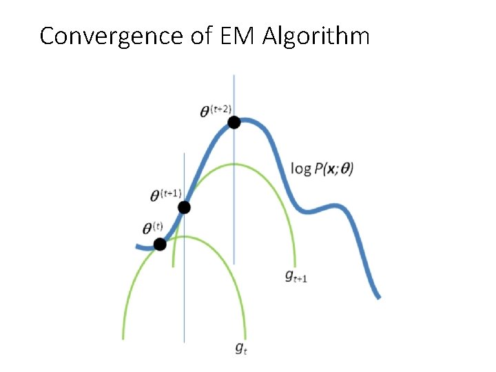
**Looking at the figure above provides a clearer and more intuitive understanding of the EM algorithm**

- Iteration \(t\):
- At time \(t\) with current parameter set \(\theta^{(t)}\), consider the lower bound **(green line)** of the log-likelihood function **(blue line)**
- During the **M-Maximization step**, maximize the lower bound and update the optimal value \(\theta^{(t+1)}\)

- Continue iteration \(t+1\) with the updated parameter set \(\theta^{(t+1)}\) from iteration \(t\) until convergence.

---

## 4. Practical Implementation

### 4.1 Implementing the GMM Using the EM Algorithm

#### 4.1 Parameter Initialization

- **mu_arr**: the array of \(k\) means of the \(k\) Gaussian distributions
- **Sigma_arr**: the array of \(k\) covariance matrices of the \(k\) Gaussian distributions
- **p_arr**: the array of \(k\) weights \(p_i\) as defined in the theoretical section
- **omega_matrix**: the matrix of \(\omega_{ij}\) as defined in the theoretical section

def _intitialize_parameters(self):
        self.mu_arr = np.asmatrix(np.random.random((self.k, self.n)) + np.mean(self.data))
        self.Sigma_arr = np.array([np.asmatrix(np.identity(self.n)) for i in range(self.k)])
        self.p_arr = np.ones(self.k) / self.k
        self.omega_matrix = np.asmatrix(np.empty((self.m, self.k)), dtype=float)

#### 4.2 E-Step – Expectation Step

**(Refer to the theoretical formulas in the previous section for the corresponding equations used in the code)**

def _expectation_step(self):
        for j in range(self.m):
            sum_density = 0
            for i in range(self.k):
                multi_normal_density = st.multivariate_normal.pdf(self.data[j, :], self.mu_arr[i].A1,
                                                                  self.Sigma_arr[i]) * self.p_arr[i]
                sum_density += multi_normal_density
                # print(multi_normal_density)
                self.omega_matrix[j, i] = multi_normal_density

            const_p_x_theta = 1 / sum_density

            self.omega_matrix[j, :] = self.omega_matrix[j, :] * const_p_x_theta
            assert self.omega_matrix[j, :].sum() - 1 < 1e-4

#### 4.3 Bước M - Maximization Step

def _maximaization_step(self):
        for i in range(self.k):
            sum_omega_for_ith_norm = self.omega_matrix[:, i].sum()
            self.p_arr[i] = 1 / self.m * sum_omega_for_ith_norm
            mu = np.zeros(self.n)
            Sigma = np.zeros((self.n, self.n))

            for j in range(self.m):
                mu += self.omega_matrix[j, i] * self.data[j, :]
                dis = (self.data[j, :] - self.mu_arr[i, :]).T * (self.data[j, :] - self.mu_arr[i, :])
                Sigma += self.omega_matrix[j, i] * dis

            self.mu_arr[i] = mu / sum_omega_for_ith_norm
            self.Sigma_arr[i] = Sigma / sum_omega_for_ith_norm

**The source code for training the model can be found [here]()**

### 4.2 Applying to a Concrete Example

**In this section, we will present only one example. For other examples, you can refer to the full source code [here]()**

In this practical example, we will reuse the dataset of **scores for the two courses: MLDM and Data Science**.

##### 4.2.1.2 Importing Required Libraries

- **pandas**: library for handling tabular data
- **numpy**: library for linear algebra operations, matrix manipulations, and vector operations
- **GMM**: package containing the GMM model and methods for plotting

import numpy as np
import pandas as pd
from GMM.GMM import *
from GMM import plot

##### 4.2.1.3 Reading the Data

mark = pd.read_csv('./ml_ds_mark.csv', sep=',', encoding='utf-8')
print("Dataset size:", mark.shape)
mark


##### 4.2.1.4 Data Preprocessing

+ Convert score ranges by taking the average

def convert_scale_2_num(scale):
    a = float(scale.split("-")[0])
    b = float(scale.split("-")[1])
    return (a + b) / 2

###### 4.2.1.5 Model Training:

def markClassification(k=2):
    x = np.array(mark_all).reshape((len(mark_all), 1))
    col_name="mark"
    legend = ["ML & DM", "Data Science", "All"]
    gmm = GMM(x, k)
    gmm.fit()
    plot.plot_1D(gmm, x, legend, col_name)

markClassification()


As we can see, our model seems to fit the data quite well for both subjects (red line). Instead of using only one normal distribution to approximate the data for the two subjects, the model has learned a mixture of two normal distributions with certain ratios (also learned by the model).

## 5 Discussion on EM and K-Means Algorithms

+ For K-means: each point undergoes a **hard assignment**, meaning that at any given time each point is assigned to only one cluster.
+ For the EM algorithm: each data point undergoes a **soft assignment**, meaning that each point is assigned probabilities of belonging to all $k$ normal distributions.


***Hình vẽ được tham khảo từ [k-means clustering](https://en.wikipedia.org/wiki/K-means_clustering)***

Looking at the figure, we see that ***both methods*** can find the ***cluster centers*** similar to the original data, however:

+ The ***K-means*** method cannot correctly capture the shape of the clusters.
+ The ***EM*** method models the shape of the data clusters much better.

***Why is that?***

Let's take another look at the probability density function:

\[
f(x_j|\mu_i, \Sigma_i) = \frac{1}{\sqrt{\det(2\pi \Sigma_i)}} \, e^{-\frac{1}{2} (x_j - \mu_i)^T \Sigma_i^{-1} (x_j - \mu_i)}
\]

If you have read the article ***[Covariance Matrix and Interesting Facts You Might Not Know]()*** on my blog, you know that ***the covariance matrix significantly affects and is closely related to the shape of the data***.

Because of this, for each data point, instead of simply computing ***Euclidean distances*** as in ***K-means***, the ***EM*** method also learns ***k covariance matrices*** for the ***k normal distributions***. Therefore, the shapes of the ***k clusters*** learned by EM describe the data better than K-means.

When the ***K-means method uses Euclidean distance***, it effectively assumes that the ***covariance matrix is the identity matrix***. As explained in ***[Covariance Matrix and Interesting Facts You Might Not Know]()***, when the ***covariance matrix is the identity matrix***, the spread along all dimensions is the same. Consequently, the shapes of the clusters learned by ***K-means*** tend to be similar in terms of form and curvature.

## 6. References

+ [k-means clustering](https://en.wikipedia.org/wiki/K-means_clustering)

+ [Appendix D - Matrix Calculus](https://ccrma.stanford.edu/~dattorro/matrixcalc.pdf)