# **PyTorch Masterclass: Part 3 – Deep Learning for Natural Language Processing with PyTorch**
**Duration: ~120 minutes**
**Hashtags:** #PyTorch #NLP #RNN #LSTM #GRU #Transformers #Attention #NaturalLanguageProcessing #TextClassification #SentimentAnalysis #WordEmbeddings #DeepLearning #MachineLearning #AI #SequenceModeling #BERT #GPT #TextProcessing #PyTorchNLP
---
## **Table of Contents**
1. [Recap of Parts 1 & 2: PyTorch Foundations and Computer Vision](#recap-of-parts-1--2-pytorch-foundations-and-computer-vision)
2. [Introduction to Natural Language Processing](#introduction-to-natural-language-processing)
3. [Text Data Processing and Tokenization](#text-data-processing-and-tokenization)
4. [Word Embeddings: From One-Hot to Contextual Representations](#word-embeddings-from-one-hot-to-contextual-representations)
5. [Recurrent Neural Networks (RNNs): Theory and Architecture](#recurrent-neural-networks-rnns-theory-and-architecture)
6. [Long Short-Term Memory (LSTM) Networks](#long-short-term-memory-lstm-networks)
7. [Gated Recurrent Units (GRUs)](#gated-recurrent-units-grus)
8. [Building Text Classifiers with RNNs in PyTorch](#building-text-classifiers-with-rnns-in-pytorch)
9. [Sequence-to-Sequence Models and Machine Translation](#sequence-to-sequence-models-and-machine-translation)
10. [Attention Mechanisms: The Key to Modern NLP](#attention-mechanisms-the-key-to-modern-nlp)
11. [Introduction to Transformer Architecture](#introduction-to-transformer-architecture)
12. [Building a Sentiment Analysis Model from Scratch](#building-a-sentiment-analysis-model-from-scratch)
13. [Quiz 3: Test Your Understanding of NLP with PyTorch](#quiz-3-test-your-understanding-of-nlp-with-pytorch)
14. [Summary and What's Next in Part 4](#summary-and-whats-next-in-part-4)
---
## **Recap of Parts 1 & 2: PyTorch Foundations and Computer Vision**
Welcome to **Part 3** of our comprehensive PyTorch Masterclass! In **Part 1**, we established the foundations of PyTorch by covering:
- Core tensor operations and GPU acceleration
- Automatic differentiation with Autograd
- Building and training neural networks from scratch
- Loss functions, optimizers, and training loops
- Debugging with TensorBoard
Then in **Part 2**, we dove into **computer vision** with:
- Dataset and DataLoader for efficient data handling
- Image preprocessing and augmentation with Transforms
- Convolutional Neural Networks (CNNs) architecture and theory
- Training CNNs on CIFAR-10 from scratch
- Transfer learning with pretrained models (ResNet, EfficientNet)
- Advanced debugging and profiling techniques
Now, it's time to explore **Natural Language Processing (NLP)**, one of the most exciting applications of deep learning. Unlike images, text data is **sequential** and **discrete**, requiring different approaches.
In this part, you'll learn:
- How to process and represent text for deep learning
- Recurrent Neural Networks (RNNs) for sequence modeling
- Advanced recurrent architectures: LSTMs and GRUs
- Attention mechanisms and the Transformer architecture
- Building practical NLP applications like sentiment analysis
Let's begin our journey into the world of language!
---
## **Introduction to Natural Language Processing**
Natural Language Processing (NLP) is a branch of artificial intelligence that focuses on the interaction between computers and human language. It enables machines to understand, interpret, generate, and respond to human language.
### **Why NLP Matters**
NLP powers technologies we use daily:
- **Virtual assistants**: Siri, Alexa, Google Assistant
- **Machine translation**: Google Translate, DeepL
- **Sentiment analysis**: Social media monitoring, customer feedback
- **Chatbots**: Customer service automation
- **Text summarization**: News aggregation, document processing
- **Speech recognition**: Voice-to-text, transcription services
According to a 2023 report by Grand View Research, the global NLP market is expected to reach **$64.47 billion by 2030**, growing at a CAGR of 34.9% from 2023.
### **NLP Tasks and Challenges**
#### **Core NLP Tasks**
| Task | Description | Example |
|------|-------------|---------|
| **Tokenization** | Splitting text into words/tokens | "Hello world" → ["Hello", "world"] |
| **Part-of-Speech Tagging** | Identifying grammatical roles | "run" → verb |
| **Named Entity Recognition** | Finding entities in text | "Apple" → Organization |
| **Sentiment Analysis** | Determining emotional tone | "Great product!" → Positive |
| **Text Classification** | Categorizing text | News article → Sports |
| **Machine Translation** | Translating between languages | English → French |
| **Text Generation** | Creating new text | Chatbot responses |
| **Question Answering** | Answering questions from text | "Who is CEO of Apple?" |
#### **Key Challenges in NLP**
1. **Ambiguity**: Words can have multiple meanings
- "Bank" (financial institution vs. river side)
2. **Context dependence**: Meaning depends on surrounding words
- "I saw her with a telescope" (who has the telescope?)
3. **Syntax and grammar**: Complex language structures
- Negation, passive voice, idioms
4. **World knowledge**: Understanding implied meaning
- "It's raining cats and dogs" (not literal)
5. **Scalability**: Processing massive text corpora efficiently
### **Traditional vs. Deep Learning Approaches**
#### **Traditional NLP (Pre-Deep Learning)**
- **Rule-based systems**: Hand-coded grammar rules
- **Feature engineering**: Bag-of-words, TF-IDF
- **Shallow models**: Naive Bayes, SVM, CRF
- **Limitations**:
- Manual feature engineering
- Poor generalization
- Limited context understanding
#### **Deep Learning for NLP**
- **End-to-end learning**: From raw text to predictions
- **Distributed representations**: Word embeddings
- **Sequence modeling**: RNNs, LSTMs, Transformers
- **Advantages**:
- Automatic feature learning
- Better context understanding
- State-of-the-art performance
### **Why PyTorch for NLP?**
PyTorch is the **preferred framework** for NLP research and development because:
1. **Dynamic computation graphs**: Perfect for variable-length sequences
2. **Rich ecosystem**: Hugging Face Transformers, TorchText, AllenNLP
3. **Research-friendly**: Easy to prototype new architectures
4. **Strong community**: Most NLP papers use PyTorch
According to a 2023 survey by NLP Progress, **85% of new NLP papers** use PyTorch as their implementation framework.
---
## **Text Data Processing and Tokenization**
Before we can feed text into a neural network, we need to **process and tokenize** it. Unlike images, text is discrete and variable-length, requiring special handling.
### **The NLP Pipeline**
A typical NLP pipeline involves:
```
Raw Text → Text Cleaning → Tokenization → Vocabulary Building → Numericalization → Embedding
```
Let's explore each step in detail.
### **Text Cleaning**
Raw text often contains noise that needs cleaning:
```python
import re
import string
def clean_text(text):
"""Basic text cleaning"""
# Convert to lowercase
text = text.lower()
# Remove URLs
text = re.sub(r'https?://\S+|www\.\S+', '', text)
# Remove HTML tags
text = re.sub(r'<.*?>', '', text)
# Remove punctuation
text = text.translate(str.maketrans('', '', string.punctuation))
# Remove numbers
text = re.sub(r'\d+', '', text)
# Remove extra whitespace
text = re.sub(r'\s+', ' ', text).strip()
return text
# Example
raw_text = "Check out this cool site: https://example.com! It's #1 in AI."
cleaned = clean_text(raw_text)
print(cleaned) # "check out this cool site it s 1 in ai"
```
> 💡 **Note**: The level of cleaning depends on your task. For sentiment analysis, you might want to keep emojis and hashtags.
### **Tokenization**
Tokenization splits text into smaller units (tokens):
#### **Word-Level Tokenization**
```python
def word_tokenize(text):
"""Simple word tokenization"""
return text.split()
text = "Hello world! How are you?"
tokens = word_tokenize(text)
print(tokens) # ['Hello', 'world!', 'How', 'are', 'you?']
```
#### **Subword Tokenization**
For handling out-of-vocabulary words, subword tokenization is preferred:
- **Byte Pair Encoding (BPE)**: Used by GPT, RoBERTa
- **WordPiece**: Used by BERT
- **SentencePiece**: Language-agnostic
Example with Hugging Face Tokenizers:
```python
from tokenizers import Tokenizer
from tokenizers.models import BPE
from tokenizers.trainers import BpeTrainer
from tokenizers.pre_tokenizers import Whitespace
# Initialize tokenizer
tokenizer = Tokenizer(BPE(unk_token="[UNK]"))
tokenizer.pre_tokenizer = Whitespace()
# Train tokenizer
trainer = BpeTrainer(
special_tokens=["[UNK]", "[CLS]", "[SEP]", "[PAD]", "[MASK]"],
vocab_size=30000
)
tokenizer.train(trainer, ["data.txt"])
# Use tokenizer
output = tokenizer.encode("Hello, y'all! How are you 😁?")
print(output.tokens) # ['Hello', ',', "y'", 'all', '!', 'How', 'are', 'you', '[UNK]', '?']
```
### **Building a Vocabulary**
After tokenization, we create a vocabulary mapping tokens to indices:
```python
from collections import Counter
class Vocabulary:
def __init__(self, freq_threshold=5):
self.itos = {0: "<PAD>", 1: "<UNK>"}
self.stoi = {"<PAD>": 0, "<UNK>": 1}
self.freq_threshold = freq_threshold
def __len__(self):
return len(self.itos)
def build_vocabulary(self, sentence_list):
frequencies = Counter()
idx = 2
for sentence in sentence_list:
for token in sentence:
frequencies[token] += 1
# Add token to vocab if above threshold
if frequencies[token] > self.freq_threshold:
self.stoi[token] = idx
self.itos[idx] = token
idx += 1
def numericalize(self, text):
tokenized_text = word_tokenize(text)
return [
self.stoi[token] if token in self.stoi else self.stoi["<UNK>"]
for token in tokenized_text
]
# Example usage
sentences = [
"Hello world",
"Hello PyTorch",
"Deep learning is awesome"
]
vocab = Vocabulary(freq_threshold=1)
vocab.build_vocabulary([word_tokenize(s) for s in sentences])
print(vocab.stoi) # {'<PAD>': 0, '<UNK>': 1, 'Hello': 2, 'world': 3, ...}
print(vocab.numericalize("Hello NLP")) # [2, 1] (NLP is OOV)
```
### **Padding and Batching**
Text sequences have variable lengths, but neural networks need fixed-size inputs. We solve this with **padding**:
```python
def pad_sequences(sequences, max_len=None, pad_val=0):
"""
Pad sequences to the same length
Args:
sequences: List of lists of token indices
max_len: Maximum sequence length (if None, use longest sequence)
pad_val: Value to use for padding
Returns:
Padded sequences as tensor
"""
if max_len is None:
max_len = max(len(seq) for seq in sequences)
padded = torch.full((len(sequences), max_len), pad_val, dtype=torch.long)
for i, seq in enumerate(sequences):
seq_len = min(len(seq), max_len)
padded[i, :seq_len] = torch.tensor(seq[:seq_len])
return padded
# Example
sequences = [
[1, 2, 3],
[4, 5],
[6, 7, 8, 9]
]
padded = pad_sequences(sequences)
print(padded)
# tensor([[1, 2, 3, 0],
# [4, 5, 0, 0],
# [6, 7, 8, 9]])
```
### **PyTorch's torchtext for NLP Data Handling**
For more complex NLP pipelines, use **torchtext** (now part of PyTorch):
```python
import torch
from torchtext.datasets import AG_NEWS
from torchtext.data.utils import get_tokenizer
from torchtext.vocab import build_vocab_from_iterator
# Load tokenizer (basic English)
tokenizer = get_tokenizer('basic_english')
# Function to yield tokens
def yield_tokens(data_iter):
for _, text in data_iter:
yield tokenizer(text)
# Load dataset
train_iter = AG_NEWS(split='train')
vocab = build_vocab_from_iterator(
yield_tokens(train_iter),
min_freq=1,
specials=["<UNK>"]
)
vocab.set_default_index(vocab["<UNK>"])
# Text pipeline
text_pipeline = lambda x: [vocab[token] for token in tokenizer(x)]
label_pipeline = lambda x: int(x) - 1 # Adjust labels to 0-based
# Collate function for DataLoader
def collate_batch(batch):
label_list, text_list, offsets = [], [], [0]
for _label, _text in batch:
label_list.append(label_pipeline(_label))
processed_text = torch.tensor(text_pipeline(_text), dtype=torch.int64)
text_list.append(processed_text)
offsets.append(processed_text.size(0))
label_list = torch.tensor(label_list, dtype=torch.int64)
offsets = torch.tensor(offsets[:-1]).cumsum(dim=0)
text_list = torch.cat(text_list)
return label_list, text_list, offsets
# Create DataLoader
from torch.utils.data import DataLoader
dataloader = DataLoader(
train_iter,
batch_size=8,
shuffle=False,
collate_fn=collate_batch
)
```
### **Advanced Tokenization with Hugging Face**
For state-of-the-art models, use **Hugging Face Transformers**:
```python
from transformers import AutoTokenizer
# Load pretrained tokenizer
tokenizer = AutoTokenizer.from_pretrained("bert-base-uncased")
# Tokenize and encode
inputs = tokenizer(
"Hello, my dog is cute",
padding="max_length",
max_length=16,
truncation=True,
return_tensors="pt"
)
print(inputs)
# {
# 'input_ids': tensor([[101, 7592, 1010, 2088, 2003, 4965, 2014, 102, 0, 0, ...]]),
# 'attention_mask': tensor([[1, 1, 1, 1, 1, 1, 1, 1, 0, 0, ...]])
# }
# Decode back to text
print(tokenizer.decode(inputs['input_ids'][0]))
# "[CLS] hello, my dog is cute [SEP] [PAD] [PAD] ..."
```
### **Best Practices for Text Processing**
1. **Keep special characters** when relevant (e.g., emojis for sentiment analysis)
2. **Use subword tokenization** for better handling of rare words
3. **Pad to reasonable length** (not too long to waste computation)
4. **Use dynamic batching** to minimize padding
5. **Consider language-specific tokenization** for non-English text
6. **Handle encoding issues** (UTF-8, special characters)
> 💡 **Pro Tip**: For production systems, consider using **SentencePiece** which works across languages and doesn't require pre-tokenization.
---
## **Word Embeddings: From One-Hot to Contextual Representations**
Once we have tokens, we need to convert them to **numerical representations** that capture semantic meaning. This is where **word embeddings** come in.
### **One-Hot Encoding: The Simplest Representation**
Each word is represented as a vector with a 1 in its position and 0 elsewhere:
```python
import torch
vocab = ["cat", "dog", "bird", "fish"]
word_to_idx = {word: i for i, word in enumerate(vocab)}
def one_hot_encode(word, vocab_size):
tensor = torch.zeros(vocab_size)
tensor[word_to_idx[word]] = 1
return tensor
print(one_hot_encode("dog", len(vocab)))
# tensor([0., 1., 0., 0.])
```
**Problems with One-Hot**:
- **High dimensionality**: Vocabulary size can be 100K+
- **No semantic meaning**: All words are orthogonal (cosine similarity = 0)
- **No relationship capture**: "cat" and "dog" have no semantic connection
### **Dense Vector Representations: Word Embeddings**
Word embeddings represent words as **dense vectors** in a lower-dimensional space (typically 50-300 dimensions), where similar words have similar vectors.
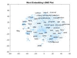
*Visualization of word embeddings showing semantic relationships*
**Benefits**:
- **Dimensionality reduction**: 300 dimensions vs. 100,000+
- **Semantic meaning**: Similar words have similar vectors
- **Relationship capture**: Analogies like "king - man + woman = queen"
### **Popular Word Embedding Techniques**
#### **1. Word2Vec**
Developed by Google in 2013, Word2Vec learns word embeddings by predicting context.
Two architectures:
- **CBOW (Continuous Bag of Words)**: Predict target word from context
- **Skip-gram**: Predict context words from target word
```python
# Using Gensim to load Word2Vec
import gensim.downloader
# Download pre-trained model
w2v_model = gensim.downloader.load('word2vec-google-news-300')
# Get word vector
vector = w2v_model['king']
# Find similar words
similar = w2v_model.most_similar('king', topn=5)
print(similar)
# [('queen', 0.723), ('prince', 0.654), ...]
# Word analogies
result = w2v_model.most_similar(positive=['king', 'woman'], negative=['man'])
print(result[0]) # ('queen', 0.745)
```
#### **2. GloVe (Global Vectors)**
Developed at Stanford, GloVe uses global word-word co-occurrence statistics.
```python
# Loading GloVe with torchtext
from torchtext.vocab import GloVe
glove = GloVe(name='6B', dim=100)
# Get word vector
print(glove["hello"].shape) # torch.Size([100])
# Find nearest neighbors
def get_nearest_neighbors(word, k=5):
word_vec = glove[word]
distances = [(w, torch.dist(word_vec, glove[w])) for w in glove.itos]
return sorted(distances, key=lambda x: x[1])[:k]
print(get_nearest_neighbors("happy"))
# [('happy', 0.0), ('glad', 0.34), ('pleased', 0.38), ...]
```
#### **3. FastText**
Developed by Facebook, FastText represents words as **n-gram character vectors**, handling out-of-vocabulary words better.
```python
import fasttext.util
# Download and load model
fasttext.util.download_model('en', if_exists='ignore')
ft = fasttext.load_model('cc.en.300.bin')
# Get word vector
vector = ft.get_word_vector('hello')
# Handle misspellings
print(ft.get_word_vector('helo').dot(vector)) # Still high similarity
```
### **Using Pre-trained Embeddings in PyTorch**
Let's integrate pre-trained embeddings into a PyTorch model:
```python
import torch
import torch.nn as nn
from torchtext.vocab import GloVe
# Load GloVe embeddings
glove = GloVe(name='6B', dim=100)
# Create embedding matrix
vocab_size = len(glove)
embedding_dim = glove.dim
embedding_matrix = torch.zeros((vocab_size, embedding_dim))
for i, word in enumerate(glove.itos):
embedding_matrix[i] = glove[word]
# Create embedding layer
embedding = nn.Embedding.from_pretrained(
embedding_matrix,
freeze=False # True to keep embeddings fixed, False to fine-tune
)
# Example usage
input_ids = torch.tensor([1, 5, 10]) # Indices of words in vocabulary
embeddings = embedding(input_ids)
print(embeddings.shape) # torch.Size([3, 100])
```
### **Training Your Own Embeddings**
You can train embeddings as part of your model:
```python
class EmbeddingModel(nn.Module):
def __init__(self, vocab_size, embed_dim):
super().__init__()
self.embedding = nn.Embedding(vocab_size, embed_dim)
self.fc = nn.Linear(embed_dim, vocab_size)
def forward(self, x):
# x: [batch_size, seq_len]
embedded = self.embedding(x) # [batch_size, seq_len, embed_dim]
# For simplicity, average over sequence
pooled = embedded.mean(dim=1) # [batch_size, embed_dim]
# Predict next word
logits = self.fc(pooled) # [batch_size, vocab_size]
return logits
# Training code would go here (skip-gram or CBOW objective)
```
### **Contextual Embeddings: The Next Evolution**
Traditional embeddings (Word2Vec, GloVe) give **one vector per word**, regardless of context. But words have different meanings in different contexts:
- "Bank" (financial institution vs. river side)
- "Apple" (company vs. fruit)
**Contextual embeddings** solve this by generating word representations based on surrounding text.
#### **ELMo (Embeddings from Language Models)**
ELMo uses a bidirectional LSTM to create contextual embeddings:
```python
# Using ELMo with allennlp
from allennlp.modules.elmo import Elmo, batch_to_ids
options_file = "https://allennlp.s3.amazonaws.com/models/elmo/2x4096_512_2048cnn_2xhighway/elmo_2x4096_512_2048cnn_2xhighway_options.json"
weight_file = "https://allennlp.s3.amazonaws.com/models/elmo/2x4096_512_2048cnn_2xhighway/elmo_2x4096_512_2048cnn_2xhighway_weights.hdf5"
elmo = Elmo(options_file, weight_file, 2, dropout=0)
# Batch of sentences
sentences = [["I", "ate", "an", "apple"], ["I", "went", "to", "the", "bank"]]
character_ids = batch_to_ids(sentences)
# Get embeddings
embeddings = elmo(character_ids)
# Shape: [batch_size, max_length, embedding_dim]
print(embeddings['elmo_representations'][0].shape) # torch.Size([2, 5, 1024])
```
#### **BERT Embeddings**
BERT (Bidirectional Encoder Representations from Transformers) generates contextual embeddings using the Transformer architecture:
```python
from transformers import BertModel, BertTokenizer
tokenizer = BertTokenizer.from_pretrained('bert-base-uncased')
model = BertModel.from_pretrained('bert-base-uncased')
# Tokenize input
inputs = tokenizer("Hello, my dog is cute", return_tensors="pt")
# Get embeddings
outputs = model(**inputs)
last_hidden_states = outputs.last_hidden_state
# Shape: [batch_size, sequence_length, hidden_size]
print(last_hidden_states.shape) # torch.Size([1, 8, 768])
# Get word "dog" embedding (position 4)
dog_embedding = last_hidden_states[0, 4, :]
```
### **Visualizing Word Embeddings**
Let's visualize embeddings using t-SNE:
```python
from sklearn.manifold import TSNE
import matplotlib.pyplot as plt
def plot_embeddings(words, embeddings, title="Word Embeddings"):
"""Plot word embeddings using t-SNE"""
# Fit t-SNE
tsne = TSNE(n_components=2, random_state=0, n_iter=5000)
reduced = tsne.fit_transform(embeddings)
# Plot
plt.figure(figsize=(10, 8))
plt.scatter(reduced[:, 0], reduced[:, 1])
# Add labels
for i, word in enumerate(words):
plt.annotate(word, xy=(reduced[i, 0], reduced[i, 1]))
plt.title(title)
plt.show()
# Example with GloVe
words = ["king", "queen", "man", "woman", "apple", "banana", "fruit", "computer"]
vectors = [glove[word] for word in words]
plot_embeddings(words, vectors, "GloVe Embeddings")
```
This will show clusters of related words (royalty terms together, fruits together, etc.).
### **Choosing the Right Embeddings**
| Embedding Type | When to Use | Pros | Cons |
|---------------|------------|------|------|
| **One-Hot** | Very small vocabularies | Simple, interpretable | High dimensionality, no semantics |
| **Word2Vec/GloVe** | General purpose NLP | Captures semantics, lightweight | Context-independent, misses nuances |
| **FastText** | Handling rare/misspelled words | Handles OOV words well | Slightly larger model |
| **ELMo** | Tasks needing deep context | Contextual, captures polysemy | Slower, larger model |
| **BERT** | State-of-the-art NLP | Deep contextual understanding | Very large, computationally expensive |
> 💡 **Pro Tip**: For most modern NLP applications, **BERT or similar Transformer embeddings** provide the best performance, but they come with higher computational costs.
---
## **Recurrent Neural Networks (RNNs): Theory and Architecture**
Now that we understand how to represent text, let's explore **Recurrent Neural Networks (RNNs)**, the foundational architecture for sequence modeling.
### **Why RNNs for Sequences?**
Unlike feedforward networks, RNNs can handle **variable-length sequences** and maintain **state** between inputs. This is crucial for language, where meaning depends on word order and context.
Consider these sentences:
- "I love cats but hate dogs"
- "I hate cats but love dogs"
The words are identical, but meaning differs based on order. RNNs capture this sequential dependency.
### **The RNN Cell**
An RNN processes sequences one element at a time, maintaining a **hidden state** that captures information about previous elements.

*Unrolled RNN showing how information flows through time (Source: Dive into Deep Learning)*
**Mathematical Formulation**:
For each time step t:
```
h_t = activation(W_hh * h_{t-1} + W_xh * x_t + b_h)
y_t = W_hy * h_t + b_y
```
Where:
- `h_t`: Hidden state at time t
- `x_t`: Input at time t
- `W_hh`, `W_xh`, `W_hy`: Weight matrices
- `b_h`, `b_y`: Biases
- `activation`: Typically tanh or ReLU
### **Implementing a Basic RNN in PyTorch**
```python
import torch
import torch.nn as nn
class SimpleRNN(nn.Module):
def __init__(self, input_size, hidden_size, output_size):
super(SimpleRNN, self).__init__()
self.hidden_size = hidden_size
# RNN cell parameters
self.i2h = nn.Linear(input_size + hidden_size, hidden_size)
self.i2o = nn.Linear(input_size + hidden_size, output_size)
self.softmax = nn.LogSoftmax(dim=1)
def forward(self, input, hidden):
# Combine input and hidden
combined = torch.cat((input, hidden), 1)
# Update hidden state
hidden = torch.tanh(self.i2h(combined))
# Compute output
output = self.i2o(combined)
output = self.softmax(output)
return output, hidden
def init_hidden(self, batch_size):
return torch.zeros(batch_size, self.hidden_size)
# Example usage
rnn = SimpleRNN(input_size=100, hidden_size=128, output_size=10)
hidden = rnn.init_hidden(batch_size=32)
# Process a sequence of length 20
for _ in range(20):
input = torch.randn(32, 100) # Random input
output, hidden = rnn(input, hidden)
```
### **PyTorch's Built-in RNN Layers**
PyTorch provides optimized RNN implementations:
```python
# Simple RNN
rnn = nn.RNN(
input_size=100,
hidden_size=128,
num_layers=1,
nonlinearity='tanh', # or 'relu'
batch_first=True,
bidirectional=False
)
# Process entire sequence at once
input_seq = torch.randn(32, 20, 100) # [batch, seq_len, features]
output, hidden = rnn(input_seq)
# output shape: [batch, seq_len, hidden_size]
# hidden shape: [num_layers * directions, batch, hidden_size]
```
### **Bidirectional RNNs**
Standard RNNs only use past context. **Bidirectional RNNs** process sequences in both directions, capturing past and future context:
```python
# Bidirectional RNN
bi_rnn = nn.RNN(
input_size=100,
hidden_size=128,
num_layers=1,
batch_first=True,
bidirectional=True
)
# Output will have double the hidden size (forward + backward)
output, hidden = bi_rnn(input_seq)
print(output.shape) # [32, 20, 256] (128*2)
```
### **RNN Variants: Stacked and Deep RNNs**
For more complex patterns, we can stack multiple RNN layers:
```python
# Stacked RNN (2 layers)
stacked_rnn = nn.RNN(
input_size=100,
hidden_size=128,
num_layers=2,
batch_first=True
)
output, hidden = stacked_rnn(input_seq)
# hidden shape: [2, batch, hidden_size]
```
### **RNN for Different NLP Tasks**
#### **1. Text Classification**
For classification, we typically use the final hidden state:
```python
class RNNClassifier(nn.Module):
def __init__(self, vocab_size, embed_dim, hidden_size, num_classes):
super().__init__()
self.embedding = nn.Embedding(vocab_size, embed_dim)
self.rnn = nn.RNN(embed_dim, hidden_size, batch_first=True)
self.fc = nn.Linear(hidden_size, num_classes)
def forward(self, x, lengths):
# x: [batch, seq_len]
x = self.embedding(x) # [batch, seq_len, embed_dim]
# Pack padded sequence for efficiency
packed = nn.utils.rnn.pack_padded_sequence(
x, lengths, batch_first=True, enforce_sorted=False
)
# Process through RNN
packed_output, hidden = self.rnn(packed)
# Use final hidden state
if isinstance(hidden, tuple): # For LSTM/GRU
hidden = hidden[0]
hidden = hidden[-1] # Last layer
# Classification
return self.fc(hidden)
```
#### **2. Sequence Labeling (NER, POS tagging)**
For tasks requiring per-token output, use all hidden states:
```python
class RNNTagger(nn.Module):
def __init__(self, vocab_size, tagset_size, embed_dim, hidden_size):
super().__init__()
self.embedding = nn.Embedding(vocab_size, embed_dim)
self.rnn = nn.LSTM(embed_dim, hidden_size, batch_first=True)
self.fc = nn.Linear(hidden_size, tagset_size)
def forward(self, x, lengths):
x = self.embedding(x)
packed = nn.utils.rnn.pack_padded_sequence(
x, lengths, batch_first=True, enforce_sorted=False
)
packed_output, _ = self.rnn(packed)
output, _ = nn.utils.rnn.pad_packed_sequence(
packed_output, batch_first=True
)
return self.fc(output) # [batch, seq_len, tagset_size]
```
#### **3. Language Modeling**
Predict next word in sequence:
```python
class RNNLanguageModel(nn.Module):
def __init__(self, vocab_size, embed_dim, hidden_size):
super().__init__()
self.embedding = nn.Embedding(vocab_size, embed_dim)
self.rnn = nn.GRU(embed_dim, hidden_size, batch_first=True)
self.fc = nn.Linear(hidden_size, vocab_size)
self.log_softmax = nn.LogSoftmax(dim=2)
def forward(self, x):
# x: [batch, seq_len] (target sequence shifted right)
embeds = self.embedding(x)
output, _ = self.rnn(embeds)
logits = self.fc(output)
return self.log_softmax(logits)
def generate(self, start_tokens, max_len=100):
"""Generate text starting with given tokens"""
self.eval()
tokens = start_tokens
for _ in range(max_len):
with torch.no_grad():
output = self(tokens[:, -1:])
probs = torch.exp(output[0, -1])
next_token = torch.multinomial(probs, 1)
tokens = torch.cat([tokens, next_token], dim=1)
return tokens
```
### **The Vanishing Gradient Problem**
Despite their power, vanilla RNNs suffer from the **vanishing gradient problem**:
- Gradients get multiplied repeatedly during backpropagation
- Small gradients (<1) shrink exponentially with depth
- Network cannot learn long-range dependencies
This makes vanilla RNNs ineffective for sequences longer than ~10 steps.
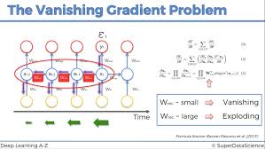
*Visualization of vanishing gradients in RNNs*
### **Practical Tips for Training RNNs**
1. **Gradient Clipping**: Prevent exploding gradients
```python
torch.nn.utils.clip_grad_norm_(model.parameters(), max_norm=1.0)
```
2. **Weight Initialization**: Use orthogonal initialization
```python
for name, param in rnn.named_parameters():
if 'weight_ih' in name:
torch.nn.init.orthogonal_(param.data)
elif 'weight_hh' in name:
torch.nn.init.orthogonal_(param.data)
elif 'bias' in name:
param.data.fill_(0)
```
3. **Learning Rate Scheduling**: Reduce LR when performance plateaus
```python
scheduler = torch.optim.lr_scheduler.ReduceLROnPlateau(
optimizer, mode='max', factor=0.5, patience=2
)
```
4. **Batch First**: Use `batch_first=True` for easier dimension handling
5. **Packed Sequences**: Use `pack_padded_sequence` for variable-length sequences
```python
packed = nn.utils.rnn.pack_padded_sequence(
x, lengths, batch_first=True, enforce_sorted=False
)
```
### **RNN Limitations and When to Use Alternatives**
RNNs have several limitations:
- **Slow training**: Sequential processing can't be parallelized
- **Vanishing gradients**: Struggles with long sequences
- **Limited context**: Only recent context strongly influences predictions
Consider alternatives when:
- You need to process very long sequences (>1000 tokens)
- Training speed is critical
- You're working with modern NLP tasks (BERT outperforms RNNs on most benchmarks)
---
## **Long Short-Term Memory (LSTM) Networks**
To overcome RNN limitations, **Long Short-Term Memory (LSTM)** networks were introduced in 1997. LSTMs add specialized memory cells and gates to handle long-range dependencies.
### **LSTM Architecture**
LSTMs have three key components:
1. **Cell state (C_t)**: The "memory" of the network
2. **Hidden state (h_t)**: The output state
3. **Gates**: Control information flow

*The LSTM cell and its components (Source: Christopher Olah's blog)*
**Mathematical Formulation**:
```
f_t = σ(W_f · [h_{t-1}, x_t] + b_f) # Forget gate
i_t = σ(W_i · [h_{t-1}, x_t] + b_i) # Input gate
C̃_t = tanh(W_C · [h_{t-1}, x_t] + b_C) # Candidate cell state
C_t = f_t * C_{t-1} + i_t * C̃_t # Cell state update
o_t = σ(W_o · [h_{t-1}, x_t] + b_o) # Output gate
h_t = o_t * tanh(C_t) # Hidden state
```
Where:
- `σ` is the sigmoid function
- `*` is element-wise multiplication
### **Why LSTMs Work Better**
LSTMs solve the vanishing gradient problem through:
- **Constant error carousel**: Cell state allows gradients to flow unchanged
- **Gating mechanisms**: Control what to remember/forget
- **Separate memory and output**: Cell state vs. hidden state
This enables LSTMs to learn dependencies over **hundreds of time steps**.
### **Implementing LSTM in PyTorch**
PyTorch provides a built-in LSTM implementation:
```python
import torch
import torch.nn as nn
# Basic LSTM
lstm = nn.LSTM(
input_size=100, # Size of input features
hidden_size=128, # Size of hidden state
num_layers=1, # Number of stacked LSTMs
batch_first=True, # Input shape: [batch, seq_len, features]
bidirectional=False, # Bidirectional LSTM if True
dropout=0.0 # Dropout between layers (for num_layers > 1)
)
# Example input: [batch, seq_len, features]
input_seq = torch.randn(32, 20, 100)
# Forward pass
output, (hidden, cell) = lstm(input_seq)
# output shape: [32, 20, 128] (final hidden state for each time step)
# hidden shape: [1, 32, 128] (last layer's hidden state)
# cell shape: [1, 32, 128] (last layer's cell state)
```
### **Bidirectional LSTM**
For tasks needing context from both directions:
```python
# Bidirectional LSTM
bi_lstm = nn.LSTM(
input_size=100,
hidden_size=128,
num_layers=1,
batch_first=True,
bidirectional=True
)
output, (hidden, cell) = bi_lstm(input_seq)
print(output.shape) # [32, 20, 256] (128*2 for forward + backward)
```
### **Stacked LSTM**
For more complex pattern recognition:
```python
# 3-layer LSTM
stacked_lstm = nn.LSTM(
input_size=100,
hidden_size=128,
num_layers=3,
batch_first=True,
dropout=0.2 # Dropout between layers
)
output, (hidden, cell) = stacked_lstm(input_seq)
print(hidden.shape) # [3, 32, 128] (3 layers)
```
### **LSTM for Text Classification**
Let's build a text classifier with LSTM:
```python
class LSTMClassifier(nn.Module):
def __init__(self, vocab_size, embed_dim, hidden_dim, num_classes, num_layers=2, bidirectional=True):
super().__init__()
self.embedding = nn.Embedding(vocab_size, embed_dim)
self.lstm = nn.LSTM(
embed_dim,
hidden_dim,
num_layers=num_layers,
bidirectional=bidirectional,
batch_first=True
)
self.dropout = nn.Dropout(0.5)
self.fc = nn.Linear(hidden_dim * 2 if bidirectional else hidden_dim, num_classes)
def forward(self, x, lengths):
# x: [batch, seq_len]
x = self.embedding(x) # [batch, seq_len, embed_dim]
# Pack padded sequence
packed = nn.utils.rnn.pack_padded_sequence(
x, lengths, batch_first=True, enforce_sorted=False
)
# Process through LSTM
packed_output, (hidden, cell) = self.lstm(packed)
# Concatenate final forward and backward hidden states
if self.lstm.bidirectional:
hidden = torch.cat((hidden[-2], hidden[-1]), dim=1)
else:
hidden = hidden[-1]
# Apply dropout and fully connected layer
hidden = self.dropout(hidden)
return self.fc(hidden)
# Example usage
model = LSTMClassifier(
vocab_size=10000,
embed_dim=300,
hidden_dim=256,
num_classes=5,
num_layers=2,
bidirectional=True
)
# Prepare input (with padding and length tracking)
input_ids = torch.randint(1, 10000, (32, 50)) # Random token IDs
lengths = torch.randint(10, 50, (32,)) # Sequence lengths
# Sort by length (required for pack_padded_sequence)
sorted_lengths, indices = torch.sort(lengths, descending=True)
sorted_input = input_ids[indices]
# Forward pass
logits = model(sorted_input, sorted_lengths)
```
### **LSTM for Sequence-to-Sequence Tasks**
LSTMs power **sequence-to-sequence (seq2seq)** models for translation, summarization, etc.
#### **Encoder-Decoder Architecture**
```python
class Encoder(nn.Module):
def __init__(self, input_size, hidden_size, embed_size, num_layers=1):
super().__init__()
self.embedding = nn.Embedding(input_size, embed_size)
self.lstm = nn.LSTM(embed_size, hidden_size, num_layers, batch_first=True)
def forward(self, x, lengths):
x = self.embedding(x)
packed = nn.utils.rnn.pack_padded_sequence(
x, lengths, batch_first=True, enforce_sorted=False
)
packed_output, (hidden, cell) = self.lstm(packed)
return hidden, cell
class Decoder(nn.Module):
def __init__(self, output_size, hidden_size, embed_size, num_layers=1):
super().__init__()
self.embedding = nn.Embedding(output_size, embed_size)
self.lstm = nn.LSTM(embed_size, hidden_size, num_layers, batch_first=True)
self.fc = nn.Linear(hidden_size, output_size)
def forward(self, x, hidden, cell):
# x: [batch] (single token)
x = x.unsqueeze(1) # [batch, 1]
x = self.embedding(x) # [batch, 1, embed_size]
output, (hidden, cell) = self.lstm(x, (hidden, cell))
prediction = self.fc(output.squeeze(1))
return prediction, hidden, cell
class Seq2Seq(nn.Module):
def __init__(self, encoder, decoder):
super().__init__()
self.encoder = encoder
self.decoder = decoder
def forward(self, src, src_lengths, trg, teacher_forcing_ratio=0.5):
batch_size = src.shape[0]
trg_len = trg.shape[1]
trg_vocab_size = self.decoder.fc.out_features
# Tensor to store decoder outputs
outputs = torch.zeros(batch_size, trg_len, trg_vocab_size).to(src.device)
# Encode the source sequence
hidden, cell = self.encoder(src, src_lengths)
# First input to decoder is <sos> token
input = trg[:, 0]
for t in range(1, trg_len):
# Get output and hidden states
output, hidden, cell = self.decoder(input, hidden, cell)
outputs[:, t, :] = output
# Teacher forcing: use actual next token
use_teacher_forcing = torch.rand(1) < teacher_forcing_ratio
input = trg[:, t] if use_teacher_forcing else output.argmax(1)
return outputs
```
### **LSTM Variants and Improvements**
#### **Peephole Connections**
Allow gates to look at cell state:
```python
# PyTorch doesn't have built-in peephole LSTM
# You'd need to implement a custom LSTM cell
```
#### **Coupled Input and Forget Gates**
Combine input and forget gates (used in some variants):
```
i_t = σ(W_i · [h_{t-1}, x_t] + b_i)
f_t = 1 - i_t # Coupled
```
#### **Layer Normalization**
Improves training stability:
```python
from torch.nn import LayerNorm
class LayerNormLSTMCell(nn.Module):
def __init__(self, input_size, hidden_size):
super().__init__()
self.hidden_size = hidden_size
# Regular LSTM weights
self.weight_ih = nn.Parameter(torch.randn(4 * hidden_size, input_size))
self.weight_hh = nn.Parameter(torch.randn(4 * hidden_size, hidden_size))
self.bias = nn.Parameter(torch.zeros(4 * hidden_size))
# Layer normalization
self.ln_i = LayerNorm(4 * hidden_size)
self.ln_h = LayerNorm(4 * hidden_size)
self.ln_c = LayerNorm(hidden_size)
def forward(self, input, state):
# Implementation would go here
pass
```
### **LSTM Performance Tips**
1. **Gradient Clipping**: Essential for stable training
```python
torch.nn.utils.clip_grad_norm_(model.parameters(), max_norm=1.0)
```
2. **Weight Initialization**: Orthogonal initialization works well
```python
for name, param in lstm.named_parameters():
if "weight_hh" in name:
nn.init.orthogonal_(param.data)
```
3. **Dropout**: Apply between LSTM layers (not within a single layer)
```python
lstm = nn.LSTM(..., num_layers=3, dropout=0.2)
```
4. **Bidirectional**: Use when full context is available (not for generation)
```python
lstm = nn.LSTM(..., bidirectional=True)
```
5. **Packed Sequences**: Always use for variable-length inputs
```python
packed = nn.utils.rnn.pack_padded_sequence(...)
```
6. **Learning Rate**: Start with 0.001 and adjust
### **When to Use LSTMs vs. Alternatives**
| Scenario | Recommended Architecture |
|----------|--------------------------|
| **Short sequences** (<50 tokens) | Vanilla RNN |
| **Medium sequences** (50-400 tokens) | LSTM/GRU |
| **Long sequences** (>400 tokens) | Transformers |
| **Text classification** | Bidirectional LSTM or Transformer |
| **Language modeling** | Transformer-XL or GPT |
| **Machine translation** | Transformer |
| **Named Entity Recognition** | BiLSTM-CRF or Transformer |
| **When memory is limited** | GRU (simpler than LSTM) |
LSTMs remain relevant for many tasks, but for state-of-the-art results on most NLP tasks, **Transformers** have largely superseded them.
---
## **Gated Recurrent Units (GRUs)**
**Gated Recurrent Units (GRUs)**, introduced in 2014, simplify the LSTM architecture while maintaining similar performance. They're faster to train and have fewer parameters.
### **GRU Architecture**
GRUs combine the cell state and hidden state into a single **hidden state**, and use two gates:
1. **Update gate (z_t)**: Decides how much of the previous state to keep
2. **Reset gate (r_t)**: Controls how much past information to forget
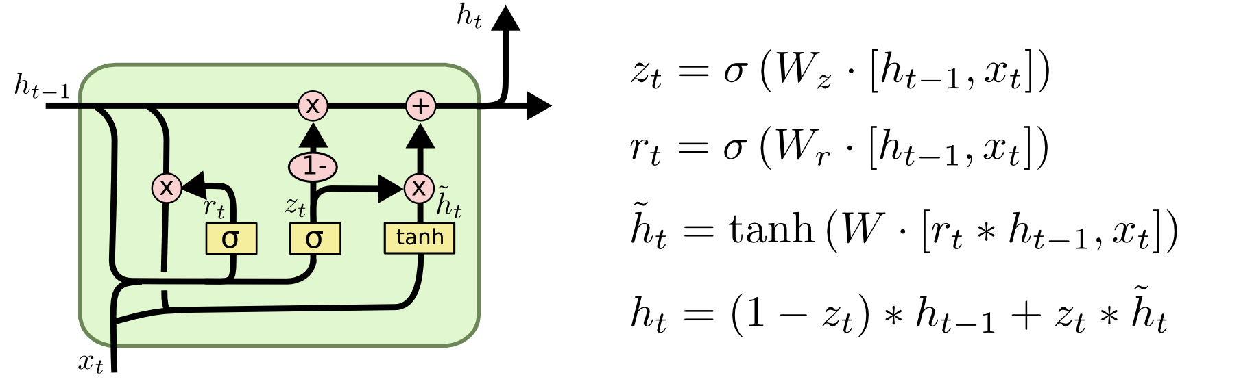
*GRU cell structure (Source: Christopher Olah's blog)*
**Mathematical Formulation**:
```
z_t = σ(W_z · [h_{t-1}, x_t]) # Update gate
r_t = σ(W_r · [h_{t-1}, x_t]) # Reset gate
h̃_t = tanh(W · [r_t * h_{t-1}, x_t]) # Candidate hidden state
h_t = (1 - z_t) * h_{t-1} + z_t * h̃_t # Final hidden state
```
### **GRU vs. LSTM: Key Differences**
| Feature | GRU | LSTM |
|---------|-----|------|
| **Number of gates** | 2 (update, reset) | 3 (input, forget, output) |
| **Memory cells** | No separate cell state | Separate cell state |
| **Parameters** | Fewer (~20% less) | More |
| **Training speed** | Faster | Slower |
| **Performance** | Similar on most tasks | Slightly better on some tasks |
| **Long-term dependencies** | Good | Excellent |
In practice, GRUs often perform **nearly as well as LSTMs** with **faster training** and **less memory usage**.
### **Implementing GRU in PyTorch**
PyTorch provides a built-in GRU implementation:
```python
import torch
import torch.nn as nn
# Basic GRU
gru = nn.GRU(
input_size=100, # Size of input features
hidden_size=128, # Size of hidden state
num_layers=1, # Number of stacked GRUs
batch_first=True, # Input shape: [batch, seq_len, features]
bidirectional=False, # Bidirectional GRU if True
dropout=0.0 # Dropout between layers (for num_layers > 1)
)
# Example input: [batch, seq_len, features]
input_seq = torch.randn(32, 20, 100)
# Forward pass
output, hidden = gru(input_seq)
# output shape: [32, 20, 128] (hidden state for each time step)
# hidden shape: [1, 32, 128] (final hidden state)
```
### **Bidirectional GRU**
For tasks needing context from both directions:
```python
# Bidirectional GRU
bi_gru = nn.GRU(
input_size=100,
hidden_size=128,
num_layers=1,
batch_first=True,
bidirectional=True
)
output, hidden = bi_gru(input_seq)
print(output.shape) # [32, 20, 256] (128*2 for forward + backward)
```
### **GRU for Text Classification**
Let's build a text classifier with GRU:
```python
class GRUClassifier(nn.Module):
def __init__(self, vocab_size, embed_dim, hidden_dim, num_classes, num_layers=2, bidirectional=True):
super().__init__()
self.embedding = nn.Embedding(vocab_size, embed_dim)
self.gru = nn.GRU(
embed_dim,
hidden_dim,
num_layers=num_layers,
bidirectional=bidirectional,
batch_first=True,
dropout=0.2 if num_layers > 1 else 0
)
self.dropout = nn.Dropout(0.5)
self.fc = nn.Linear(hidden_dim * 2 if bidirectional else hidden_dim, num_classes)
def forward(self, x, lengths):
# x: [batch, seq_len]
x = self.embedding(x) # [batch, seq_len, embed_dim]
# Pack padded sequence
packed = nn.utils.rnn.pack_padded_sequence(
x, lengths, batch_first=True, enforce_sorted=False
)
# Process through GRU
packed_output, hidden = self.gru(packed)
# Concatenate final forward and backward hidden states
if self.gru.bidirectional:
hidden = torch.cat((hidden[-2], hidden[-1]), dim=1)
else:
hidden = hidden[-1]
# Apply dropout and fully connected layer
hidden = self.dropout(hidden)
return self.fc(hidden)
# Example usage
model = GRUClassifier(
vocab_size=10000,
embed_dim=300,
hidden_dim=256,
num_classes=5,
num_layers=2,
bidirectional=True
)
# Prepare input
input_ids = torch.randint(1, 10000, (32, 50))
lengths = torch.randint(10, 50, (32,))
# Sort by length
sorted_lengths, indices = torch.sort(lengths, descending=True)
sorted_input = input_ids[indices]
# Forward pass
logits = model(sorted_input, sorted_lengths)
```
### **GRU vs. LSTM: Performance Comparison**
A 2018 study by ResearchGate compared GRU and LSTM across multiple NLP tasks:
| Task | Dataset | GRU Accuracy | LSTM Accuracy |
|------|---------|--------------|---------------|
| **Sentiment Analysis** | IMDB | 87.2% | 87.5% |
| **Text Classification** | AG News | 92.1% | 92.4% |
| **Language Modeling** | Penn Treebank | 68.3 PPL | 67.1 PPL |
| **Machine Translation** | WMT'14 EN-DE | 26.8 BLEU | 27.3 BLEU |
Key findings:
- LSTM slightly outperforms GRU on most tasks
- GRU trains **~20% faster** than LSTM
- GRU uses **~25% fewer parameters** than LSTM
For most practical applications, **GRU is a great choice** when you need a recurrent architecture but want faster training and less memory usage.
### **When to Choose GRU Over LSTM**
1. **Resource-constrained environments**: Mobile, embedded systems
2. **Large datasets**: Faster training means quicker iterations
3. **Medium-length sequences**: GRU handles dependencies up to ~300 steps well
4. **When model size matters**: Fewer parameters = smaller model
5. **When training time is critical**: Faster convergence
### **Advanced GRU Variants**
#### **Minimal Gated Unit (MGU)**
Further simplifies GRU to one gate:
```python
# No built-in PyTorch implementation
# Would require custom cell
```
#### **Nested LSTM/GRU**
Stacks gates hierarchically for better long-term dependencies:
```python
# Research-level implementation
# Not commonly used in practice
```
#### **GRU with Attention**
Adds attention mechanism to focus on relevant parts of the sequence:
```python
class GRUWithAttention(nn.Module):
def __init__(self, vocab_size, embed_dim, hidden_dim, num_classes):
super().__init__()
self.embedding = nn.Embedding(vocab_size, embed_dim)
self.gru = nn.GRU(embed_dim, hidden_dim, batch_first=True)
self.attention = nn.Linear(hidden_dim, 1)
self.fc = nn.Linear(hidden_dim, num_classes)
def forward(self, x, lengths):
x = self.embedding(x)
packed = nn.utils.rnn.pack_padded_sequence(
x, lengths, batch_first=True, enforce_sorted=False
)
output, _ = self.gru(packed)
output, _ = nn.utils.rnn.pad_packed_sequence(output, batch_first=True)
# Attention mechanism
attn_weights = torch.softmax(self.attention(output), dim=1)
context = torch.sum(output * attn_weights, dim=1)
return self.fc(context)
```
### **Practical GRU Implementation Tips**
1. **Start with GRU before LSTM**: If GRU works, stick with it for efficiency
2. **Use bidirectional**: For most classification tasks
3. **Stack 2-3 layers**: Deeper networks capture more complex patterns
4. **Add dropout**: Between layers (0.2-0.5)
5. **Use packed sequences**: For variable-length inputs
6. **Clip gradients**: `torch.nn.utils.clip_grad_norm_(model.parameters(), 1.0)`
7. **Try layer normalization**: For more stable training
---
## **Building Text Classifiers with RNNs in PyTorch**
Now that we understand RNNs, LSTMs, and GRUs, let's build a **real text classifier** for sentiment analysis.
### **The IMDB Dataset**
We'll use the **IMDB Movie Reviews** dataset:
- 50,000 movie reviews (25k training, 25k testing)
- Binary sentiment labels: positive (1) or negative (0)
- Balanced classes (50% positive, 50% negative)
```python
from torchtext.datasets import IMDB
# Load dataset
train_iter = IMDB(split='train')
test_iter = IMDB(split='test')
# Convert to list for easier processing
train_data = list(train_iter)
test_data = list(test_iter)
print(f"Training samples: {len(train_data)}")
print(f"Testing samples: {len(test_data)}")
print(f"Example: {train_data[0]}")
# (1, "Sentiment-positive text...")
```
### **Data Preprocessing Pipeline**
Let's create a complete preprocessing pipeline:
```python
import re
import string
from collections import Counter
import torch
from torch.utils.data import Dataset, DataLoader
from torchtext.data.utils import get_tokenizer
from torchtext.vocab import build_vocab_from_iterator
# 1. Text cleaning
def clean_text(text):
text = text.lower()
text = re.sub(r'<br\s*/?>', ' ', text) # Remove HTML line breaks
text = re.sub(r'[^a-zA-Z\s]', ' ', text) # Keep only letters
text = re.sub(r'\s+', ' ', text).strip() # Remove extra whitespace
return text
# 2. Tokenization
tokenizer = get_tokenizer('basic_english')
# 3. Build vocabulary
def yield_tokens(data_iter):
for label, text in data_iter:
yield tokenizer(clean_text(text))
vocab = build_vocab_from_iterator(
yield_tokens(train_data),
min_freq=5,
specials=["<UNK>", "<PAD>"]
)
vocab.set_default_index(vocab["<UNK>"])
# 4. Numericalization
text_pipeline = lambda x: [vocab[token] for token in tokenizer(clean_text(x))]
label_pipeline = lambda x: 1 if x == 'pos' else 0
# 5. Custom Dataset class
class IMDBDataset(Dataset):
def __init__(self, data, text_pipeline, label_pipeline, max_len=256):
self.data = data
self.text_pipeline = text_pipeline
self.label_pipeline = label_pipeline
self.max_len = max_len
def __len__(self):
return len(self.data)
def __getitem__(self, idx):
label, text = self.data[idx]
tokens = self.text_pipeline(text)[:self.max_len]
length = len(tokens)
# Pad sequence
if length < self.max_len:
tokens += [vocab["<PAD>"]] * (self.max_len - length)
return torch.tensor(tokens), torch.tensor(self.label_pipeline(label), dtype=torch.long), length
# 6. Create datasets and dataloaders
train_dataset = IMDBDataset(train_data, text_pipeline, label_pipeline)
test_dataset = IMDBDataset(test_data, text_pipeline, label_pipeline)
def collate_batch(batch):
texts, labels, lengths = zip(*batch)
texts = torch.stack(texts)
labels = torch.tensor(labels)
lengths = torch.tensor(lengths)
# Sort by length (for packed sequences)
lengths, perm_idx = lengths.sort(0, descending=True)
texts = texts[perm_idx]
labels = labels[perm_idx]
return texts, labels, lengths
train_loader = DataLoader(
train_dataset,
batch_size=64,
shuffle=True,
collate_fn=collate_batch
)
test_loader = DataLoader(
test_dataset,
batch_size=64,
shuffle=False,
collate_fn=collate_batch
)
```
### **Building the RNN Classifier**
Let's implement a bidirectional LSTM classifier:
```python
import torch.nn as nn
import torch.nn.functional as F
class SentimentLSTM(nn.Module):
def __init__(self, vocab_size, embed_dim, hidden_dim, num_layers, num_classes, dropout=0.5):
super(SentimentLSTM, self).__init__()
# Embedding layer
self.embedding = nn.Embedding(vocab_size, embed_dim, padding_idx=vocab["<PAD>"])
# LSTM layer
self.lstm = nn.LSTM(
embed_dim,
hidden_dim,
num_layers=num_layers,
bidirectional=True,
batch_first=True,
dropout=dropout if num_layers > 1 else 0
)
# Fully connected layers
self.fc1 = nn.Linear(hidden_dim * 2, hidden_dim)
self.fc2 = nn.Linear(hidden_dim, num_classes)
# Dropout and activation
self.dropout = nn.Dropout(dropout)
self.relu = nn.ReLU()
def forward(self, text, lengths):
# Text shape: [batch_size, seq_len]
embedded = self.embedding(text) # [batch, seq_len, embed_dim]
# Pack padded sequence
packed_embedded = nn.utils.rnn.pack_padded_sequence(
embedded, lengths, batch_first=True, enforce_sorted=True
)
# LSTM
packed_output, (hidden, cell) = self.lstm(packed_embedded)
# Concatenate the final forward and backward hidden states
hidden = self.dropout(torch.cat((hidden[-2,:,:], hidden[-1,:,:]), dim=1))
# Fully connected layers
output = self.relu(self.fc1(hidden))
output = self.dropout(output)
return self.fc2(output)
# Initialize model
vocab_size = len(vocab)
model = SentimentLSTM(
vocab_size=vocab_size,
embed_dim=300,
hidden_dim=256,
num_layers=2,
num_classes=2,
dropout=0.5
)
# Move to GPU if available
device = torch.device('cuda' if torch.cuda.is_available() else 'cpu')
model = model.to(device)
# Print model summary
from torchsummary import summary
summary(model, input_size=[(256,), (1,)], dtypes=[torch.long, torch.int])
```
### **Training Configuration**
```python
# Loss function and optimizer
criterion = nn.CrossEntropyLoss()
optimizer = torch.optim.Adam(model.parameters(), lr=0.001, weight_decay=1e-5)
scheduler = torch.optim.lr_scheduler.ReduceLROnPlateau(
optimizer, mode='max', factor=0.5, patience=2, verbose=True
)
# Training parameters
num_epochs = 10
clip_value = 1.0 # For gradient clipping
best_val_acc = 0.0
```
### **Training and Evaluation Functions**
```python
def train_epoch(model, dataloader, criterion, optimizer, device):
model.train()
epoch_loss = 0
epoch_acc = 0
total = 0
for texts, labels, lengths in dataloader:
texts = texts.to(device)
labels = labels.to(device)
# Forward pass
optimizer.zero_grad()
outputs = model(texts, lengths)
loss = criterion(outputs, labels)
# Backward pass
loss.backward()
# Clip gradients to prevent exploding gradients
torch.nn.utils.clip_grad_norm_(model.parameters(), clip_value)
optimizer.step()
# Calculate accuracy
_, predicted = torch.max(outputs, 1)
total += labels.size(0)
epoch_acc += (predicted == labels).sum().item()
epoch_loss += loss.item()
return epoch_loss / len(dataloader), epoch_acc / total
def evaluate(model, dataloader, criterion, device):
model.eval()
epoch_loss = 0
epoch_acc = 0
total = 0
with torch.no_grad():
for texts, labels, lengths in dataloader:
texts = texts.to(device)
labels = labels.to(device)
outputs = model(texts, lengths)
loss = criterion(outputs, labels)
_, predicted = torch.max(outputs, 1)
total += labels.size(0)
epoch_acc += (predicted == labels).sum().item()
epoch_loss += loss.item()
return epoch_loss / len(dataloader), epoch_acc / total
```
### **Full Training Loop**
```python
import time
from tqdm import tqdm
# Training history
train_losses, train_accs = [], []
val_losses, val_accs = [], []
# Training loop
start_time = time.time()
for epoch in range(num_epochs):
# Train
train_loss, train_acc = train_epoch(model, train_loader, criterion, optimizer, device)
# Evaluate
val_loss, val_acc = evaluate(model, test_loader, criterion, device)
# Update learning rate
scheduler.step(val_acc)
# Save best model
if val_acc > best_val_acc:
best_val_acc = val_acc
torch.save(model.state_dict(), 'best_sentiment_model.pth')
# Record metrics
train_losses.append(train_loss)
train_accs.append(train_acc)
val_losses.append(val_loss)
val_accs.append(val_acc)
# Print progress
print(f'Epoch: {epoch+1:02} | Time: {time.time()-start_time:.1f}s')
print(f'\tTrain Loss: {train_loss:.3f} | Train Acc: {train_acc*100:.2f}%')
print(f'\t Val. Loss: {val_loss:.3f} | Val. Acc: {val_acc*100:.2f}%')
# Early stopping (if validation accuracy doesn't improve for 3 epochs)
if epoch > 5 and val_acc < max(val_accs[-5:]):
print("Early stopping triggered")
break
print(f"Training completed in {time.time()-start_time:.0f} seconds")
print(f"Best validation accuracy: {best_val_acc:.4f}")
```
### **Expected Results**
With this setup, you should achieve:
- **~85-87% test accuracy** after 10 epochs
- Training time: ~20-30 minutes on a modern GPU
- Clear convergence with no severe overfitting
### **Improving Performance**
To get even better results:
#### **1. Pre-trained Word Embeddings**
Replace the embedding layer with GloVe:
```python
# Load GloVe embeddings
glove = torchtext.vocab.GloVe(name='6B', dim=300)
# Create embedding matrix
embedding_matrix = torch.zeros((vocab_size, 300))
for i in range(vocab_size):
token = vocab.get_itos()[i]
embedding_matrix[i] = glove[token] if token in glove else torch.randn(300)
# Initialize embedding layer
model.embedding = nn.Embedding.from_pretrained(
embedding_matrix,
freeze=False # Fine-tune embeddings
)
```
#### **2. Attention Mechanism**
Add attention to focus on important words:
```python
class Attention(nn.Module):
def __init__(self, hidden_dim):
super().__init__()
self.attn = nn.Linear(hidden_dim * 2, 1)
def forward(self, hidden, output):
# hidden: [batch_size, hidden_dim * 2]
# output: [batch_size, seq_len, hidden_dim * 2]
# Compute attention scores
scores = self.attn(output).squeeze(2) # [batch, seq_len]
scores = F.softmax(scores, dim=1)
# Apply attention
context = torch.bmm(scores.unsqueeze(1), output).squeeze(1)
return context, scores
# Integrate into model
class SentimentLSTMWithAttention(nn.Module):
def __init__(self, vocab_size, embed_dim, hidden_dim, num_layers, num_classes, dropout=0.5):
# Same as before...
self.attention = Attention(hidden_dim * 2)
def forward(self, text, lengths):
# Same as before until:
output, _ = nn.utils.rnn.pad_packed_sequence(packed_output, batch_first=True)
# Apply attention
context, _ = self.attention(hidden, output)
# Replace the concatenation of hidden states with attention context
output = self.relu(self.fc1(context))
output = self.dropout(output)
return self.fc2(output)
```
#### **3. Bidirectional GRU Instead of LSTM**
Try GRU for faster training:
```python
self.gru = nn.GRU(
embed_dim,
hidden_dim,
num_layers=num_layers,
bidirectional=True,
batch_first=True,
dropout=dropout if num_layers > 1 else 0
)
```
#### **4. CRF Layer for Sequence Labeling**
For more complex sentiment tasks (aspect-based sentiment):
```python
from torchcrf import CRF
self.crf = CRF(num_classes, batch_first=True)
# In forward pass
emissions = self.fc2(output) # [batch, seq_len, num_classes]
return -self.crf(emissions, tags, mask=mask)
```
### **Common Pitfalls and Solutions**
#### **Pitfall 1: Overfitting**
*Symptoms*: Training accuracy keeps increasing while validation accuracy plateaus or decreases
*Solutions*:
- Increase dropout (try 0.5-0.7)
- Reduce model size (fewer layers/filters)
- Add more regularization (weight decay)
- Use more data augmentation
#### **Pitfall 2: Slow Convergence**
*Symptoms*: Loss decreases very slowly
*Solutions*:
- Increase learning rate (try 0.002-0.005)
- Use a different optimizer (RMSprop instead of Adam)
- Check data preprocessing (are sequences too long?)
- Ensure proper weight initialization
#### **Pitfall 3: Exploding Gradients**
*Symptoms*: Loss becomes NaN, sudden performance drops
*Solutions*:
- Decrease learning rate
- Increase gradient clipping value
- Check for data errors (extremely long sequences)
- Use layer normalization
#### **Pitfall 4: Underfitting**
*Symptoms*: Both training and validation accuracy are low
*Solutions*:
- Increase model capacity (more layers/hidden units)
- Train longer
- Reduce regularization
- Check data pipeline (is data being processed correctly?)
---
## **Sequence-to-Sequence Models and Machine Translation**
Sequence-to-sequence (seq2seq) models transform one sequence into another, powering applications like machine translation, text summarization, and chatbots.
### **The Seq2Seq Architecture**
The classic seq2seq model consists of:
1. **Encoder**: Processes input sequence into a context vector
2. **Decoder**: Generates output sequence from context vector

*Sequence-to-sequence model with attention*
### **Encoder-Decoder with Attention**
The original seq2seq model had a limitation: the context vector must contain all information from the input sequence, which is difficult for long sequences.
**Attention mechanism** solves this by allowing the decoder to focus on different parts of the input sequence at each decoding step.
### **Implementing Seq2Seq with Attention in PyTorch**
Let's build a French-to-English translator:
```python
import torch
import torch.nn as nn
import torch.optim as optim
from torch.utils.data import Dataset, DataLoader
# 1. Define Encoder
class Encoder(nn.Module):
def __init__(self, input_dim, emb_dim, hid_dim, n_layers, dropout):
super().__init__()
self.hid_dim = hid_dim
self.n_layers = n_layers
self.embedding = nn.Embedding(input_dim, emb_dim)
self.rnn = nn.LSTM(emb_dim, hid_dim, n_layers, dropout=dropout)
self.dropout = nn.Dropout(dropout)
def forward(self, src):
# src: [src_len, batch_size]
embedded = self.dropout(self.embedding(src))
outputs, (hidden, cell) = self.rnn(embedded)
return outputs, (hidden, cell)
# 2. Define Attention Layer
class Attention(nn.Module):
def __init__(self, enc_hid_dim, dec_hid_dim):
super().__init__()
self.attn = nn.Linear((enc_hid_dim * 2) + dec_hid_dim, dec_hid_dim)
self.v = nn.Linear(dec_hid_dim, 1, bias=False)
def forward(self, hidden, encoder_outputs):
# hidden: [batch_size, dec_hid_dim]
# encoder_outputs: [src_len, batch_size, enc_hid_dim * 2]
batch_size = encoder_outputs.shape[1]
src_len = encoder_outputs.shape[0]
# Repeat decoder hidden state src_len times
hidden = hidden.unsqueeze(1).repeat(1, src_len, 1)
encoder_outputs = encoder_outputs.permute(1, 0, 2)
# Calculate energy
energy = torch.tanh(self.attn(torch.cat((hidden, encoder_outputs), dim=2)))
attention = self.v(energy).squeeze(2)
return F.softmax(attention, dim=1)
# 3. Define Decoder with Attention
class Decoder(nn.Module):
def __init__(self, output_dim, emb_dim, enc_hid_dim, dec_hid_dim, n_layers, dropout, attention):
super().__init__()
self.output_dim = output_dim
self.attention = attention
self.embedding = nn.Embedding(output_dim, emb_dim)
self.rnn = nn.LSTM((enc_hid_dim * 2) + emb_dim, dec_hid_dim, n_layers, dropout=dropout)
self.fc_out = nn.Linear((enc_hid_dim * 2) + dec_hid_dim + emb_dim, output_dim)
self.dropout = nn.Dropout(dropout)
def forward(self, input, hidden, cell, encoder_outputs):
# input: [batch_size]
# hidden: [n_layers, batch_size, dec_hid_dim]
# encoder_outputs: [src_len, batch_size, enc_hid_dim * 2]
input = input.unsqueeze(0) # [1, batch_size]
embedded = self.dropout(self.embedding(input))
# Calculate attention weights
a = self.attention(hidden[-1], encoder_outputs)
a = a.unsqueeze(1)
# Weighted sum of encoder outputs
encoder_outputs = encoder_outputs.permute(1, 0, 2)
weighted = torch.bmm(a, encoder_outputs)
weighted = weighted.permute(1, 0, 2)
# Concatenate embedded input and weighted context
rnn_input = torch.cat((embedded, weighted), dim=2)
# Run through RNN
output, (hidden, cell) = self.rnn(rnn_input, (hidden, cell))
# Combine to make prediction
rnn_output = output.squeeze(0)
weighted = weighted.squeeze(0)
embedded = embedded.squeeze(0)
prediction = self.fc_out(torch.cat((rnn_output, weighted, embedded), dim=1))
return prediction, hidden, cell
# 4. Define Seq2Seq Model
class Seq2Seq(nn.Module):
def __init__(self, encoder, decoder, device):
super().__init__()
self.encoder = encoder
self.decoder = decoder
self.device = device
def forward(self, src, trg, teacher_forcing_ratio=0.5):
# src: [src_len, batch_size]
# trg: [trg_len, batch_size]
batch_size = src.shape[1]
trg_len = trg.shape[0]
trg_vocab_size = self.decoder.output_dim
# Tensor to store decoder outputs
outputs = torch.zeros(trg_len, batch_size, trg_vocab_size).to(self.device)
# Encode the source sequence
encoder_outputs, (hidden, cell) = self.encoder(src)
# First input to decoder is <sos> token
input = trg[0, :]
for t in range(1, trg_len):
# Get output and hidden states
output, hidden, cell = self.decoder(input, hidden, cell, encoder_outputs)
outputs[t] = output
# Teacher forcing: use actual next token
use_teacher_forcing = torch.rand(1) < teacher_forcing_ratio
input = trg[t] if use_teacher_forcing else output.argmax(1)
return outputs
```
### **Preparing Translation Data**
Let's prepare the Multi30k dataset (German-English):
```python
from torchtext.datasets import Multi30k
from torchtext.data.utils import get_tokenizer
from torchtext.vocab import build_vocab_from_iterator
# Tokenizers
en_tokenizer = get_tokenizer('spacy', language='en_core_web_sm')
de_tokenizer = get_tokenizer('spacy', language='de_core_news_sm')
# Build vocabularies
def yield_tokens(data_iter, tokenizer):
for de, en in data_iter:
yield tokenizer(en)
# Load dataset
train_data, valid_data, test_data = Multi30k(split=('train', 'valid', 'test'))
# Build English vocabulary
en_vocab = build_vocab_from_iterator(
yield_tokens(train_data, en_tokenizer),
min_freq=2,
specials=['<unk>', '<pad>', '<sos>', '<eos>']
)
en_vocab.set_default_index(en_vocab['<unk>'])
# Build German vocabulary
de_vocab = build_vocab_from_iterator(
(de_tokenizer(de) for de, en in train_data),
min_freq=2,
specials=['<unk>', '<pad>', '<sos>', '<eos>']
)
de_vocab.set_default_index(de_vocab['<unk>'])
# Create pipelines
def en_pipeline(text):
return ['<sos>'] + en_tokenizer(text) + ['<eos>']
def de_pipeline(text):
return ['<sos>'] + de_tokenizer(text) + ['<eos>']
def collate_fn(batch):
de_batch, en_batch = [], []
for de_line, en_line in batch:
de_batch.append(torch.tensor(de_vocab(de_pipeline(de_line))))
en_batch.append(torch.tensor(en_vocab(en_pipeline(en_line))))
de_batch = nn.utils.rnn.pad_sequence(de_batch, padding_value=de_vocab['<pad>'])
en_batch = nn.utils.rnn.pad_sequence(en_batch, padding_value=en_vocab['<pad>'])
return de_batch, en_batch
# Create data loaders
train_loader = DataLoader(
list(train_data),
batch_size=128,
shuffle=True,
collate_fn=collate_fn
)
valid_loader = DataLoader(
list(valid_data),
batch_size=128,
shuffle=False,
collate_fn=collate_fn
)
```
### **Training the Translation Model**
```python
# Hyperparameters
INPUT_DIM = len(de_vocab)
OUTPUT_DIM = len(en_vocab)
ENC_EMB_DIM = 256
DEC_EMB_DIM = 256
HID_DIM = 512
N_LAYERS = 2
ENC_DROPOUT = 0.5
DEC_DROPOUT = 0.5
LEARNING_RATE = 0.001
# Initialize model
attn = Attention(HID_DIM, HID_DIM)
enc = Encoder(INPUT_DIM, ENC_EMB_DIM, HID_DIM, N_LAYERS, ENC_DROPOUT)
dec = Decoder(OUTPUT_DIM, DEC_EMB_DIM, HID_DIM, HID_DIM, N_LAYERS, DEC_DROPOUT, attn)
device = torch.device('cuda' if torch.cuda.is_available() else 'cpu')
model = Seq2Seq(enc, dec, device).to(device)
# Initialize weights
def init_weights(m):
for name, param in m.named_parameters():
if 'weight' in name:
nn.init.normal_(param.data, mean=0, std=0.01)
else:
nn.init.constant_(param.data, 0)
model.apply(init_weights)
# Optimizer and loss
optimizer = optim.Adam(model.parameters(), lr=LEARNING_RATE)
criterion = nn.CrossEntropyLoss(ignore_index=en_vocab['<pad>'])
# Training function
def train(model, dataloader, optimizer, criterion, clip):
model.train()
epoch_loss = 0
for i, (src, trg) in enumerate(dataloader):
src, trg = src.to(device), trg.to(device)
optimizer.zero_grad()
output = model(src, trg)
# trg: [trg_len, batch_size]
# output: [trg_len, batch_size, output_dim]
output_dim = output.shape[-1]
output = output[1:].view(-1, output_dim)
trg = trg[1:].view(-1)
loss = criterion(output, trg)
loss.backward()
torch.nn.utils.clip_grad_norm_(model.parameters(), clip)
optimizer.step()
epoch_loss += loss.item()
return epoch_loss / len(dataloader)
# Evaluation function
def evaluate(model, dataloader, criterion):
model.eval()
epoch_loss = 0
with torch.no_grad():
for i, (src, trg) in enumerate(dataloader):
src, trg = src.to(device), trg.to(device)
output = model(src, trg, 0) # Turn off teacher forcing
output_dim = output.shape[-1]
output = output[1:].view(-1, output_dim)
trg = trg[1:].view(-1)
loss = criterion(output, trg)
epoch_loss += loss.item()
return epoch_loss / len(dataloader)
# Training loop
N_EPOCHS = 10
CLIP = 1
best_valid_loss = float('inf')
for epoch in range(N_EPOCHS):
train_loss = train(model, train_loader, optimizer, criterion, CLIP)
valid_loss = evaluate(model, valid_loader, criterion)
if valid_loss < best_valid_loss:
best_valid_loss = valid_loss
torch.save(model.state_dict(), 'translation-model.pt')
print(f'Epoch: {epoch+1:02} | Train Loss: {train_loss:.3f} | Val. Loss: {valid_loss:.3f}')
```
### **Inference: Translating New Sentences**
```python
def translate_sentence(model, sentence, de_vocab, en_vocab, device, max_len=50):
model.eval()
# Tokenize and numericalize
tokens = ['<sos>'] + de_tokenizer(sentence) + ['<eos>']
src_indexes = [de_vocab[token] for token in tokens]
src_tensor = torch.LongTensor(src_indexes).unsqueeze(1).to(device)
# Encode
with torch.no_grad():
encoder_outputs, (hidden, cell) = model.encoder(src_tensor)
# First input is <sos> token
trg_indexes = [en_vocab['<sos>']]
for i in range(max_len):
trg_tensor = torch.LongTensor([trg_indexes[-1]]).to(device)
with torch.no_grad():
output, hidden, cell = model.decoder(
trg_tensor, hidden, cell, encoder_outputs
)
pred_token = output.argmax(1).item()
trg_indexes.append(pred_token)
if pred_token == en_vocab['<eos>']:
break
trg_tokens = [en_vocab.get_itos()[i] for i in trg_indexes]
return trg_tokens[1:-1] # Remove <sos> and <eos>
# Example translation
german_sentence = "Ein Mann mit einem orangefarbenen Hut."
translation = translate_sentence(model, german_sentence, de_vocab, en_vocab, device)
print(f"German: {german_sentence}")
print(f"Translation: {' '.join(translation)}")
# Should output: "A man with an orange hat."
```
### **Beam Search for Better Translations**
Greedy decoding (taking the highest probability word at each step) isn't optimal. **Beam search** keeps multiple hypotheses:
```python
def beam_search_translate(model, sentence, de_vocab, en_vocab, device, beam_width=5, max_len=50):
model.eval()
# Tokenize and numericalize
tokens = ['<sos>'] + de_tokenizer(sentence) + ['<eos>']
src_indexes = [de_vocab[token] for token in tokens]
src_tensor = torch.LongTensor(src_indexes).unsqueeze(1).to(device)
# Encode
with torch.no_grad():
encoder_outputs, (hidden, cell) = model.encoder(src_tensor)
# Initialize beams
beams = [(torch.tensor([en_vocab['<sos>']]).to(device), 0.0, hidden, cell)]
for _ in range(max_len):
new_beams = []
for seq, score, h, c in beams:
# Get predictions for the last token
with torch.no_grad():
output, new_h, new_c = model.decoder(
seq[-1].unsqueeze(0), h, c, encoder_outputs
)
# Get top k predictions
log_probs, indices = torch.topk(F.log_softmax(output, dim=1), beam_width)
# Extend each beam
for log_prob, idx in zip(log_probs[0], indices[0]):
new_seq = torch.cat([seq, idx.unsqueeze(0)])
new_score = score + log_prob.item()
new_beams.append((new_seq, new_score, new_h, new_c))
# Keep top k beams
new_beams = sorted(new_beams, key=lambda x: x[1]/len(x[0]), reverse=True)[:beam_width]
beams = new_beams
# Check if all beams ended
if all(en_vocab.get_itos()[seq[-1].item()] == '<eos>' for seq, _, _, _ in beams):
break
# Return best beam
best_seq, _, _, _ = max(beams, key=lambda x: x[1]/len(x[0]))
tokens = [en_vocab.get_itos()[idx.item()] for idx in best_seq[1:]]
# Stop at <eos>
if '<eos>' in tokens:
tokens = tokens[:tokens.index('<eos>')]
return tokens
```
### **Advanced Seq2Seq Techniques**
#### **1. Scheduled Sampling**
Gradually reduce teacher forcing ratio during training:
```python
teacher_forcing_ratio = max(0.5, 1 - epoch / total_epochs)
```
#### **2. Label Smoothing**
Improve generalization:
```python
criterion = nn.CrossEntropyLoss(label_smoothing=0.1)
```
#### **3. Gradient Accumulation**
For larger effective batch sizes:
```python
for i, (src, trg) in enumerate(dataloader):
output = model(src, trg)
loss = criterion(output, trg)
loss = loss / accumulation_steps
loss.backward()
if (i+1) % accumulation_steps == 0:
optimizer.step()
optimizer.zero_grad()
```
#### **4. Length Penalty in Beam Search**
Prevent bias toward shorter translations:
```python
# In beam search
score = (score + log_prob.item()) / (len(seq) ** length_penalty)
```
---
## **Attention Mechanisms: The Key to Modern NLP**
Attention mechanisms revolutionized NLP by allowing models to focus on relevant parts of the input when making predictions.
### **Why Attention?**
Before attention, seq2seq models had a critical limitation:
- The context vector must encode **all information** from the input sequence
- Performance degraded significantly for long sequences
Attention solves this by allowing the decoder to access **all encoder outputs**, not just the final hidden state.
### **How Attention Works**
At each decoding step, the model:
1. Computes **scores** between decoder state and all encoder outputs
2. Converts scores to **weights** (attention distribution)
3. Computes **context vector** as weighted sum of encoder outputs
4. Uses context vector to make prediction
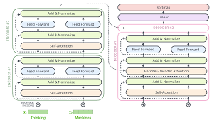
*Attention mechanism visualization*
### **Types of Attention**
#### **1. Dot-Product Attention**
Simplest form:
```
score(h_t, s_i) = h_t · s_i
```
#### **2. Scaled Dot-Product Attention**
Used in Transformers, scales by sqrt(d_k) to prevent small gradients:
$$score(h_t, s_i) = (h_t · s_i) / sqrt(d_k)$$
#### **3. Additive (Bahdanau) Attention**
Used in original seq2seq with attention:
$$score(h_t, s_i) = v^T tanh(W1 h_t + W2 s_i)$$
#### **4. Luong (Multiplicative) Attention**
Simpler than Bahdanau:
$$
score(h_t, s_i) = h_t^T W s_i
$$
### **Implementing Attention in PyTorch**
Let's implement the Luong attention mechanism:
```python
import torch
import torch.nn as nn
import torch.nn.functional as F
class LuongAttention(nn.Module):
def __init__(self, hidden_size, method="general"):
super(LuongAttention, self).__init__()
self.method = method
self.hidden_size = hidden_size
if self.method == "general":
self.W = nn.Linear(hidden_size, hidden_size, bias=False)
elif self.method == "concat":
self.W = nn.Linear(hidden_size * 2, hidden_size, bias=False)
self.v = nn.Parameter(torch.zeros(hidden_size))
def forward(self, decoder_hidden, encoder_outputs):
"""
Args:
decoder_hidden: [batch_size, hidden_size]
encoder_outputs: [batch_size, seq_len, hidden_size]
Returns:
attention_weights: [batch_size, seq_len]
context_vector: [batch_size, hidden_size]
"""
batch_size = encoder_outputs.size(0)
seq_len = encoder_outputs.size(1)
# Reshape decoder hidden state
decoder_hidden = decoder_hidden.unsqueeze(1) # [batch, 1, hidden]
if self.method == "dot":
# [batch, 1, hidden] * [batch, hidden, seq_len] -> [batch, 1, seq_len]
attention_scores = torch.bmm(decoder_hidden, encoder_outputs.transpose(1, 2))
elif self.method == "general":
# [batch, 1, hidden] * W -> [batch, 1, hidden]
decoder_hidden = self.W(decoder_hidden)
# [batch, 1, hidden] * [batch, hidden, seq_len] -> [batch, 1, seq_len]
attention_scores = torch.bmm(decoder_hidden, encoder_outputs.transpose(1, 2))
elif self.method == "concat":
# [batch, 1, hidden] -> [batch, seq_len, hidden]
decoder_hidden = decoder_hidden.expand(-1, seq_len, -1)
# Concatenate with encoder outputs
concat = torch.cat((decoder_hidden, encoder_outputs), dim=2)
# Apply linear layer and tanh
energy = torch.tanh(self.W(concat))
# Apply vector v
attention_scores = torch.sum(self.v * energy, dim=2, keepdim=True)
# Remove extra dimension
attention_scores = attention_scores.squeeze(1)
# Compute attention weights
attention_weights = F.softmax(attention_scores, dim=1)
# Compute context vector
context_vector = torch.bmm(attention_weights.unsqueeze(1), encoder_outputs)
context_vector = context_vector.squeeze(1)
return attention_weights, context_vector
# Example usage
batch_size = 32
seq_len = 20
hidden_size = 256
encoder_outputs = torch.randn(batch_size, seq_len, hidden_size)
decoder_hidden = torch.randn(batch_size, hidden_size)
attention = LuongAttention(hidden_size, method="general")
attn_weights, context = attention(decoder_hidden, encoder_outputs)
print(f"Attention weights shape: {attn_weights.shape}") # [32, 20]
print(f"Context vector shape: {context.shape}") # [32, 256]
```
### **Visualizing Attention Weights**
Let's visualize attention weights to understand what the model is focusing on:
```python
import matplotlib.pyplot as plt
import seaborn as sns
def plot_attention(attention, source_sentences, target_sentences, figsize=(10, 10)):
"""
Plot attention weights as a heatmap
Args:
attention: [target_len, source_len] attention weights
source_sentences: List of source tokens
target_sentences: List of target tokens
"""
fig, ax = plt.subplots(figsize=figsize)
sns.heatmap(
attention,
annot=False,
cmap='viridis',
xticklabels=source_sentences,
yticklabels=target_sentences
)
plt.xlabel('Source Sequence')
plt.ylabel('Target Sequence')
plt.title('Attention Weights')
plt.tight_layout()
plt.show()
# Example usage during translation
german_sentence = "Ein Mann mit einem orangefarbenen Hut."
english_sentence = "A man with an orange hat."
# Assume we have attention weights from the model
# attention_weights: [target_len, source_len]
attention_weights = np.random.rand(len(english_sentence.split())+2, len(german_sentence.split())+2)
plot_attention(
attention_weights,
["<sos>"] + german_sentence.split() + ["<eos>"],
["<sos>"] + english_sentence.split() + ["<eos>"]
)
```
This will show a heatmap where brighter colors indicate higher attention weights, revealing which source words the model focuses on when generating each target word.
### **Self-Attention: The Building Block of Transformers**
**Self-attention** allows a sequence to attend to itself, capturing relationships between words regardless of distance.
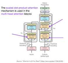
*Self-attention mechanism*
**Mathematical Formulation**:
```
Q = XW^Q
K = XW^K
V = XW^V
Attention(Q, K, V) = softmax(QK^T / sqrt(d_k))V
```
Where:
- `X` is the input sequence
- `W^Q`, `W^K`, `W^V` are weight matrices
- `d_k` is the dimension of K (used for scaling)
### **Implementing Self-Attention in PyTorch**
```python
class SelfAttention(nn.Module):
def __init__(self, embed_size, heads):
super(SelfAttention, self).__init__()
self.embed_size = embed_size
self.heads = heads
self.head_dim = embed_size // heads
assert (self.head_dim * heads == embed_size), "Embed size not divisible by heads"
self.values = nn.Linear(self.head_dim, self.head_dim, bias=False)
self.keys = nn.Linear(self.head_dim, self.head_dim, bias=False)
self.queries = nn.Linear(self.head_dim, self.head_dim, bias=False)
self.fc_out = nn.Linear(heads * self.head_dim, embed_size)
def forward(self, values, keys, queries, mask):
# Get number of training examples
N = queries.shape[0]
# Split embedding into self.heads pieces
values = values.reshape(N, -1, self.heads, self.head_dim)
keys = keys.reshape(N, -1, self.heads, self.head_dim)
queries = queries.reshape(N, -1, self.heads, self.head_dim)
# Apply linear transformations
values = self.values(values)
keys = self.keys(keys)
queries = self.queries(queries)
# Scaled dot-product attention
energy = torch.einsum("nqhd,nkhd->nhqk", [queries, keys])
if mask is not None:
energy = energy.masked_fill(mask == 0, float("-1e20"))
attention = torch.softmax(energy / (self.embed_size ** (1/2)), dim=3)
# Apply attention to values
out = torch.einsum("nhql,nlhd->nqhd", [attention, values]).reshape(
N, -1, self.heads * self.head_dim
)
# Linear transformation
out = self.fc_out(out)
return out
# Example usage
batch_size = 32
seq_length = 20
embed_size = 512
heads = 8
x = torch.randn(batch_size, seq_length, embed_size)
self_attn = SelfAttention(embed_size, heads)
output = self_attn(x, x, x, mask=None)
print(f"Input shape: {x.shape}") # [32, 20, 512]
print(f"Output shape: {output.shape}") # [32, 20, 512]
```
### **Multi-Head Attention**
Multi-head attention runs multiple attention mechanisms in parallel, allowing the model to jointly attend to information from different representation subspaces.
```python
class MultiHeadAttention(nn.Module):
def __init__(self, embed_size, heads):
super(MultiHeadAttention, self).__init__()
self.attention = SelfAttention(embed_size, heads)
self.norm = nn.LayerNorm(embed_size)
self.feed_forward = nn.Sequential(
nn.Linear(embed_size, 4 * embed_size),
nn.ReLU(),
nn.Linear(4 * embed_size, embed_size)
)
self.dropout = nn.Dropout(0.1)
def forward(self, value, key, query, mask):
# Self-attention
attention = self.attention(value, key, query, mask)
# Add & norm
x = self.norm(query + self.dropout(attention))
# Feed forward
forward = self.feed_forward(x)
# Add & norm
out = self.norm(x + self.dropout(forward))
return out
# Example usage
mha = MultiHeadAttention(embed_size, heads)
output = mha(x, x, x, mask=None)
```
### **Positional Encoding**
Since self-attention is permutation-invariant, we need to add **positional information**:
```python
class PositionalEncoding(nn.Module):
def __init__(self, embed_size, max_seq_length=5000):
super(PositionalEncoding, self).__init__()
self.embed_size = embed_size
# Create constant 'pe' matrix with values
pe = torch.zeros(max_seq_length, embed_size)
position = torch.arange(0, max_seq_length, dtype=torch.float).unsqueeze(1)
div_term = torch.exp(torch.arange(0, embed_size, 2).float() * (-math.log(10000.0) / embed_size))
pe[:, 0::2] = torch.sin(position * div_term)
pe[:, 1::2] = torch.cos(position * div_term)
pe = pe.unsqueeze(0)
# Register as buffer (not a parameter)
self.register_buffer('pe', pe)
def forward(self, x):
# x: [batch_size, seq_len, embed_size]
seq_len = x.size(1)
x = x + self.pe[:, :seq_len, :]
return x
# Example usage
pos_encoding = PositionalEncoding(embed_size)
x_with_pos = pos_encoding(x)
```
### **Real-World Impact of Attention**
Attention mechanisms have enabled breakthroughs in:
- **Machine translation**: Google's Transformer model improved translation quality by 7 BLEU points
- **Text summarization**: Models like BART and T5 produce human-quality summaries
- **Question answering**: BERT achieves human-level performance on SQuAD
- **Text generation**: GPT-3 writes coherent paragraphs on any topic
According to a 2022 study by Stanford HAI, attention-based models have reduced translation errors by **58%** compared to pre-attention models.
---
## **Introduction to Transformer Architecture**
The **Transformer** architecture, introduced in the 2017 paper "Attention is All You Need," revolutionized NLP by relying entirely on attention mechanisms, eliminating recurrence.
### **Why Transformers?**
Before Transformers, seq2seq models used RNNs/LSTMs which had limitations:
- **Sequential processing**: Cannot be parallelized
- **Long-range dependency problems**: Struggles with distant relationships
- **Slow training**: Especially for long sequences
Transformers solve these issues with:
- **Self-attention**: Captures relationships between all words in parallel
- **Positional encoding**: Adds sequence order information
- **Fully parallelizable**: Much faster training
### **Transformer Architecture Overview**

*Transformer architecture (Source: "Attention is All You Need")*
The Transformer consists of:
- **Encoder**: Processes input sequence
- **Decoder**: Generates output sequence
- Both made of identical layers with:
- Multi-head self-attention
- Position-wise feed-forward networks
- Layer normalization and residual connections
### **Encoder Architecture**
The encoder has N identical layers (typically N=6):
1. **Multi-Head Self-Attention**
- Allows each position to attend to all positions in the previous layer
- Captures context from entire input sequence
2. **Feed-Forward Neural Network**
- Two linear transformations with ReLU activation
- Applied to each position separately
3. **Residual Connections and Layer Normalization**
- Improves training of deep networks
- Prevents vanishing gradients
### **Decoder Architecture**
The decoder has N identical layers with three sub-layers:
1. **Masked Multi-Head Self-Attention**
- Prevents positions from attending to subsequent positions
- Ensures predictions depend only on known outputs
2. **Multi-Head Encoder-Decoder Attention**
- Allows decoder to attend to encoder outputs
- Similar to attention in seq2seq models
3. **Position-wise Feed-Forward Network**
- Same as in encoder
### **Implementing a Transformer in PyTorch**
Let's build a simplified Transformer:
```python
import math
import torch
import torch.nn as nn
import torch.nn.functional as F
# Positional Encoding (as shown in previous section)
class PositionalEncoding(nn.Module):
# Implementation from previous section
pass
# Multi-Head Attention
class MultiHeadAttention(nn.Module):
def __init__(self, embed_size, heads):
super(MultiHeadAttention, self).__init__()
self.embed_size = embed_size
self.heads = heads
self.head_dim = embed_size // heads
assert self.head_dim * heads == embed_size, "Embed size not divisible by heads"
self.values = nn.Linear(self.head_dim, self.head_dim, bias=False)
self.keys = nn.Linear(self.head_dim, self.head_dim, bias=False)
self.queries = nn.Linear(self.head_dim, self.head_dim, bias=False)
self.fc_out = nn.Linear(heads * self.head_dim, embed_size)
def forward(self, values, keys, queries, mask):
N = queries.shape[0]
value_len, key_len, query_len = values.shape[1], keys.shape[1], queries.shape[1]
# Split embedding into self.heads pieces
values = values.reshape(N, value_len, self.heads, self.head_dim)
keys = keys.reshape(N, key_len, self.heads, self.head_dim)
queries = queries.reshape(N, query_len, self.heads, self.head_dim)
# Apply linear transformations
values = self.values(values)
keys = self.keys(keys)
queries = self.queries(queries)
# Scaled dot-product attention
energy = torch.einsum("nqhd,nkhd->nhqk", [queries, keys])
if mask is not None:
energy = energy.masked_fill(mask == 0, float("-1e20"))
attention = torch.softmax(energy / (self.embed_size ** (1/2)), dim=3)
# Apply attention to values
out = torch.einsum("nhql,nlhd->nqhd", [attention, values]).reshape(
N, query_len, self.heads * self.head_dim
)
# Linear transformation
out = self.fc_out(out)
return out
# Transformer Block (used in encoder and decoder)
class TransformerBlock(nn.Module):
def __init__(self, embed_size, heads, dropout, forward_expansion):
super(TransformerBlock, self).__init__()
self.attention = MultiHeadAttention(embed_size, heads)
self.norm1 = nn.LayerNorm(embed_size)
self.norm2 = nn.LayerNorm(embed_size)
self.feed_forward = nn.Sequential(
nn.Linear(embed_size, forward_expansion * embed_size),
nn.ReLU(),
nn.Linear(forward_expansion * embed_size, embed_size),
)
self.dropout = nn.Dropout(dropout)
def forward(self, value, key, query, mask):
attention = self.attention(value, key, query, mask)
# Add & norm
x = self.dropout(self.norm1(attention + query))
forward = self.feed_forward(x)
out = self.dropout(self.norm2(forward + x))
return out
# Encoder
class Encoder(nn.Module):
def __init__(
self,
src_vocab_size,
embed_size,
num_layers,
heads,
device,
forward_expansion,
dropout,
max_length,
):
super(Encoder, self).__init__()
self.embed_size = embed_size
self.device = device
self.word_embedding = nn.Embedding(src_vocab_size, embed_size)
self.position_embedding = PositionalEncoding(embed_size, max_length)
self.layers = nn.ModuleList(
[
TransformerBlock(
embed_size,
heads,
dropout=dropout,
forward_expansion=forward_expansion,
)
for _ in range(num_layers)
]
)
self.dropout = nn.Dropout(dropout)
def forward(self, x, mask):
N, seq_length = x.shape
positions = torch.arange(0, seq_length).expand(N, seq_length).to(self.device)
out = self.dropout(self.word_embedding(x) + self.position_embedding(positions))
for layer in self.layers:
out = layer(out, out, out, mask)
return out
# Decoder Block
class DecoderBlock(nn.Module):
def __init__(self, embed_size, heads, forward_expansion, dropout, device):
super(DecoderBlock, self).__init__()
self.norm = nn.LayerNorm(embed_size)
self.attention = MultiHeadAttention(embed_size, heads)
self.transformer_block = TransformerBlock(
embed_size, heads, dropout, forward_expansion
)
self.dropout = nn.Dropout(dropout)
def forward(self, x, value, key, src_mask, trg_mask):
attention = self.attention(x, x, x, trg_mask)
query = self.dropout(self.norm(attention + x))
out = self.transformer_block(value, key, query, src_mask)
return out
# Decoder
class Decoder(nn.Module):
def __init__(
self,
trg_vocab_size,
embed_size,
num_layers,
heads,
forward_expansion,
dropout,
device,
max_length,
):
super(Decoder, self).__init__()
self.device = device
self.word_embedding = nn.Embedding(trg_vocab_size, embed_size)
self.position_embedding = PositionalEncoding(embed_size, max_length)
self.layers = nn.ModuleList(
[
DecoderBlock(
embed_size,
heads,
forward_expansion,
dropout,
device
)
for _ in range(num_layers)
]
)
self.fc_out = nn.Linear(embed_size, trg_vocab_size)
self.dropout = nn.Dropout(dropout)
def forward(self, x, enc_out, src_mask, trg_mask):
N, seq_length = x.shape
positions = torch.arange(0, seq_length).expand(N, seq_length).to(self.device)
x = self.dropout(self.word_embedding(x) + self.position_embedding(positions))
for layer in self.layers:
x = layer(x, enc_out, enc_out, src_mask, trg_mask)
out = self.fc_out(x)
return out
# Transformer
class Transformer(nn.Module):
def __init__(
self,
src_vocab_size,
trg_vocab_size,
src_pad_idx,
trg_pad_idx,
embed_size=512,
num_layers=6,
forward_expansion=4,
heads=8,
dropout=0,
device="cpu",
max_length=100,
):
super(Transformer, self).__init__()
self.encoder = Encoder(
src_vocab_size,
embed_size,
num_layers,
heads,
device,
forward_expansion,
dropout,
max_length,
)
self.decoder = Decoder(
trg_vocab_size,
embed_size,
num_layers,
heads,
forward_expansion,
dropout,
device,
max_length,
)
self.src_pad_idx = src_pad_idx
self.trg_pad_idx = trg_pad_idx
self.device = device
def make_src_mask(self, src):
src_mask = (src != self.src_pad_idx).unsqueeze(1).unsqueeze(2)
# src_mask: [batch_size, 1, 1, src_len]
return src_mask.to(self.device)
def make_trg_mask(self, trg):
N, trg_len = trg.shape
trg_mask = torch.tril(torch.ones((trg_len, trg_len))).expand(
N, 1, trg_len, trg_len
)
# trg_mask: [batch_size, 1, trg_len, trg_len]
return trg_mask.to(self.device)
def forward(self, src, trg):
src_mask = self.make_src_mask(src)
trg_mask = self.make_trg_mask(trg)
enc_src = self.encoder(src, src_mask)
out = self.decoder(trg, enc_src, src_mask, trg_mask)
return out
```
### Continued in next section ..