# **WEEK 6**
# **[Day 1: K-Nearest Neighbor & SVM](https://colab.research.google.com/drive/1iB_zPIooGev3ngUIvPAHEsicvdpm3ilT?usp=sharing)**
## **Bias-Variance trade-off**
**Total error:**
$$
Err(x) = \mathrm{Bias}^2 + \mathrm{Variance} + \mathrm{Irreducible\ Error}
$$
Bias:
- Is error from erroneous assumptions in the learning algorithm.
- the average of all predictions
- High bias: underfitting. The predictions are no way near the label, model could be too simple
- Low bias: model can predict well
Variance:
- Is error from sensitivity to small fluctuations in the training set
- Testing the sensitivity of the model to changes.
- Low variance: change data point, model a bit -> prediction should not be changing much
- High variance: change model a bit -> predictions change a lot
Noise: irreducible error, is the noise term in the true relationship that cannot fundamentally be reduced by any model.
<img src="https://i.imgur.com/ssAwUQc.png" width="50%"/>
The usual analogy is target shooting or archery.
High bias is equivalent to aiming in the wrong place. High variance is equivalent to having an unsteady aim.
This can lead to the following scenarios:
* Low bias, low variance: Aiming at the target and hitting it with good precision.
* Low bias, high variance: Aiming at the target, but not hitting it consistently.
* High bias, low variance: Aiming off the target, but being consistent.
* High bias, high variance: Aiming off the target and being inconsistent.
**Low bias Low variance: ideal model**
Low bias, High variance => Overfitting
High bias, Low variance => Underfitting
High bias high variance

==**Detecting High Bias and High Variance**==
**High Bias**: *Training error is high*
* Use more complex model (e.g. kernel methods)
* Adding features (more columns)
**High Variance**: *Training error is much lower than test error*
* Add more training data
* Reduce the model complexity (e.g. Regularization)
## **Regulaziration**
Preventing the model to be overcomplex therefore overfitting.
For linear model, regularization is typically achieved by penalizing large individual weights. A regularization term is added to the cost funnction.
By adding a regularization term to the loss function, we are trying to achieve 2 goals at once:
- We try to fit the training data well (by keep small loss)
- We try to keep the weights small so no weight (weights) will stand out and cause overfitting
L2: squared all weights (Ridge)
L1: absolute values of weight (Lasso)
Elastic Net: both L1 and L2 (adjusting to get the best fit to our data set)

* alpha 0: no regularization, still overfitting
* alpha too small: Overfitting
* alpha too big: underfitting
=> How to choose the good lamda: trying a range from 0 to 10 and compare errors on test set
hyperparameter vs parameters (weights):
hyperparameter: is chosen by hooman (alpha, max_iter, solver, fit_intercept,...)
## **K-Nearest Neighbors**
**Assumption: Similar inputs must have similar output.**
Can use for classification(by choosing the label of the majority) and regression problems (by calculating the average of the neighbors)
K: number of neighbors -> majority is which color? -> determine the color of the white point -> prediction
<div align="center">
<img src="https://i.imgur.com/TO1HvCA.png" />
<div>
No weight, no bias -> nothing to update, just looking at the dataset and find the neighbors
Weakness: dataset is huge -> slow because it proposional to the size of dataset, it has to search in the whole dataset to find
- Parametric models have the advantage of often being faster to predict, but the disadvantage of making stronger assumptions about the data distribution.
- Non-parametric models are more flexible, but often computationally expensive.
**The distance function**
distance between 2 points
Using L1 and L2
* **$p=1$**, **Manhattan distance**, or **$L_1$ distance**, or **$L_1$ norm**
$$
dist(x, x') = \sum_{i=1}^{n}{|x_i - x'_i|}
$$
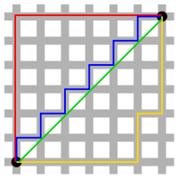
* **$p=2$**, **Euclidean distance**, or **$L_2$ distance**, or **$L_2$ norm**
$$
dist(x, x') = \sqrt{\sum_{i=1}^{n}{(x_i - x'_i)^2}}
$$

L2 is shorter than L1.
Small K: overfitting (too sensitive to changes (adding more data points) and outliers)
Bigger K: reducing the complexity and sensitivity. Too big: Underfitting
**K-fold cross validation**
To find a good ML model, we need to evaluate our model carefully. In k-fold cross validation, we randomly split the training dataset into k folds without replacement, where 𝑘−1 folds are used for the model training, and one fold is used for performance evaluation. We do that k times to obtain k models and performance estimates. Then we calculate the average performance of the models. Typically, we use k-fold cross validation for hyperparameter tuning.
Do K times validation test. Split the dataset into K pieces.
=> take average validation errors

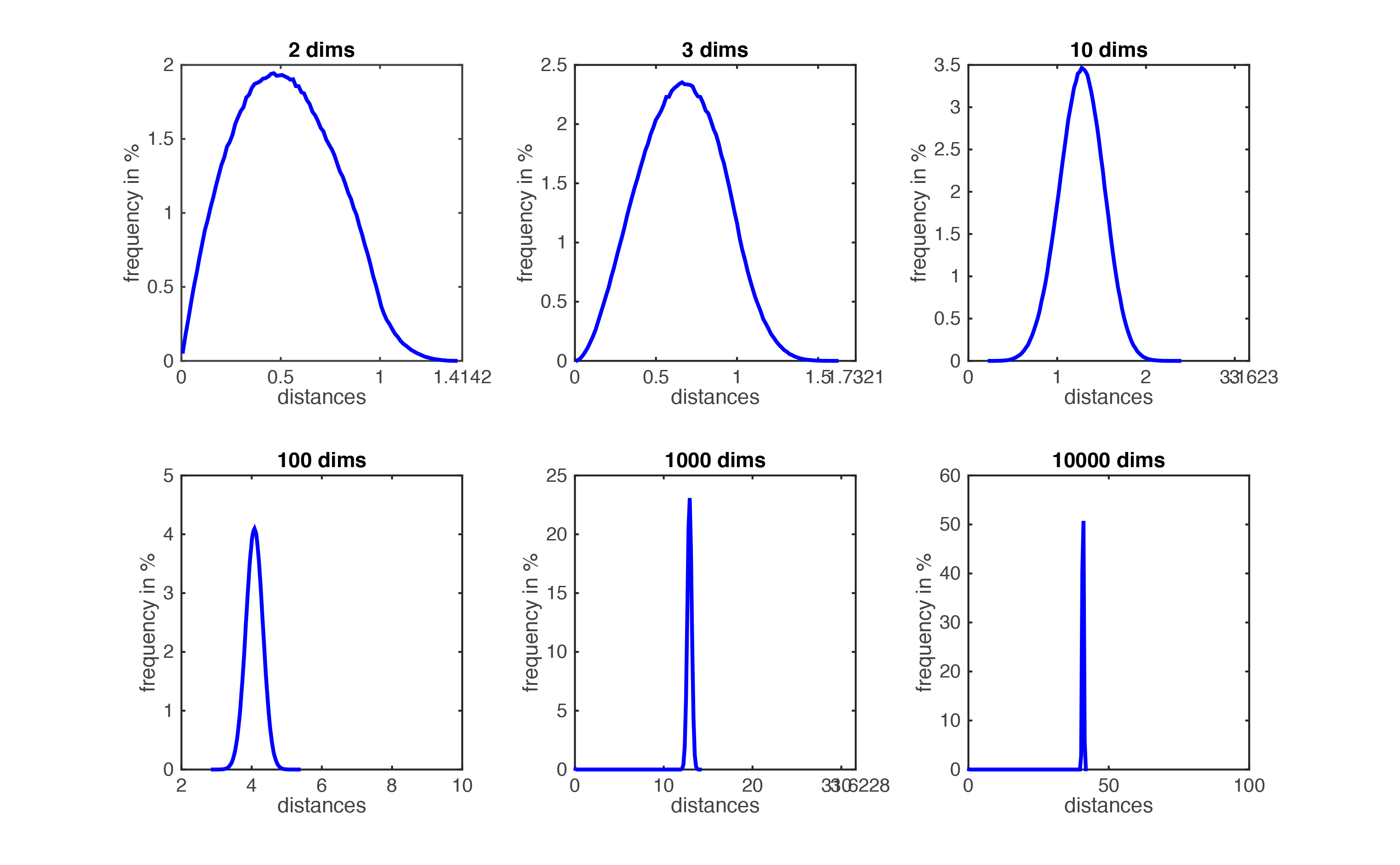
**Curse of Dimensionality**
In high dimension space, data points (rows in dataset) ten to be far to each other. This problem is known as the **curse of dimensionality**.
When number of features (p) is large, and dataset size (n) is still the same, KNN performs worst because curse of dimensionality: That is, K observations that are nearest to a given test observation x0 (when p is small) may be very far away from x0 in p-dimensional space (when p is increased)
=> meaning there will be very few neighbor observations “near” any given observation when we increase # of features.
=> in theory, the distance between points is much less meaningful in large dimensions
**Bonus**: This is not true for deep learning
In high dimensionality applications deep learning does not suffer from the same consequences as other machine learning algorithms such as Linear Regression or KNN.
This fact is part of the magic that makes this methodology of modeling with Neural Networks so effective. Neural Network’s imperviousness to the curse of dimensionality is a helpful characteristic in today’s world of big data.
https://hackernoon.com/what-killed-the-curse-of-dimensionality-8dbfad265bbe
## **Support Vector Machine**
For classification problems
To find the maximum **margin** to seperate classes
Look for nearest points of each class to the decision boundary -> the distance is called margin -> we need to maximize both distances
Return the min of all distance from all data points to hyperplane.
$$
\Rightarrow
\gamma(\mathbf{w},b)=\min_{\mathbf{x}\in D}\frac{\left | \mathbf{w}^T\mathbf{x}+b \right |}{\left \| \mathbf{w} \right \|_{2}}
$$
Step:
Calculate the gamma for each class (the margin -> gind the minimum margin -> the distance between the closest data point)
Next step: How to maximize the margin ?
The data has to be linearly separated and all the data points must lie on the correct side of the hyperlane.
Hard margin:
at 1 y(wTx +b)
# **Day 2: SVM - Kernel SVM - Decision Tree - Bagging and Boosting**
## **[SVM](https://colab.research.google.com/drive/11RO7vVMfdbLXfqQTkA_KqITe49i4h0hi?usp=sharing)**
Good for classification problems
Find the closest points of each side to the hyperplane and maximize the distances. Those distances have to be **equal** and the **biggest** -> only one solution
Margin: the distance from the closest points to the hyperplane
$$
\Rightarrow
\gamma(\mathbf{w},b)=\min_{\mathbf{x}\in D}\frac{\left | \mathbf{w}^T\mathbf{x}+b \right |}{\left \| \mathbf{w} \right \|_{2}}
$$
=> Maximize the margins
The objective is to maximize the margin under the contraints that all data points must lie on the correct side of the hyperplane
$$
\underbrace{\max_{\mathbf{w},b}\gamma(\mathbf{w},b)}_{maximize \ margin} \textrm{such that} \ \ \underbrace{\forall i \ y^{(i)}(\mathbf{w}^Tx^{(i)}+b)\geq 0}_{separating \ hyperplane}
$$
...
$$
\begin{align}
&\min_{\mathbf{w},b}\mathbf{w}^T\mathbf{w}&\\
&\textrm{s.t.} \ \ \ \forall i \ y^{(i)}(\mathbf{w}^T \mathbf{x}^{(i)}+b) \geq 1 &
\end{align}
$$
| y (true label) | wx + b | y*(wx+b) | correct prediction? |
|--|--|--|--|
| 1| >=1|>=1 | **yes**|
|1 | <-1 |<-1 | no|
|-1| >=1 | <-1 | no|
|-1| <-1 |>=1 | **yes**|
=> Set the margins to 1
However, hard-margin SVM tends to be too sensitive to certain new data point
**The support vector**
For the optimal $\mathbf{w},b$, some training points will have tight contraints. Must satisfy this condition: (y is 1 or -1)
$$
y^{(i)}(\mathbf{w}^T \mathbf{x}^{(i)}+b) = 1.
$$
Every points line on the line (boundaries) is called support vectors
(point that makes the result > 1 or -1 will be inside the boundaries)
Weakness: kind of overfitting problems. Model is too sensitive to changes (adding one more data point) -> soft margin
SVC: kernel=linear
**Soft margin**
Allow some points to be in between the margins. -> use different points to define margin. => generalize better => prevent overfitting => change C from 10 to 0.1 in SVC
What is C?
-> A way (hyperparameter) to penalize the points in between the margins, big C + more points in between -> that term is big -> the loss is bigger because that function is to determine the loss.
Very big C -> underfitting
Try a range of C to find the lowest error (for loop [0.001, 0.01, 0.1, 1, 10])
$$
\min_{\mathbf{w},b}\underbrace{\mathbf{w}^T\mathbf{w}}_{l_{2}-regularizer} + C\ \sum_{i=1}^{m}\underbrace{\max\left [ 1-y^{(i)}(\mathbf{w}^T \mathbf{x}^{(i)}+b),0 \right ]}_{hinge-loss}
$$
Correlation of Support vector and hyperplane when increasing or decreasing C???
## **[Kernel SVM](https://colab.research.google.com/drive/1V1CyC8BLV0w35Ac8v5-35I3wEzSuKqU5?usp=sharing)**
==When hyperplane is not a straight/linear line==
==Projecting on a higher dimension (adding more columns) -> separate by a hyperplane -> project back into 2D -> create a decision boundary==
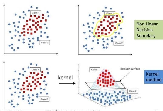
**The kernel trick**
**Lagrange multiplier**
find a way to combine into one formular
$$
\begin{align}
&\min_{\mathbf{w},b}\mathbf{w}^T\mathbf{w}&\\
&\textrm{s.t.} \ \ \ \ y^{(i)}(\mathbf{w}^T \mathbf{x}^{(i)}+b) = 1 &
\end{align}
$$
=>
$$
\mathcal{L} = \frac{1}{2} \mathbf{w}^T\mathbf{w} - \sum{\lambda^{(i)} \big( y^{(i)}( \mathbf{w}^T \mathbf{x}^{(i)}+b) - 1 \big)}
$$
=> minimize the equation above -> take derivative of that and set = 0
Our expression becomes (the loss function that we want to minimize):
$$\begin{align}
\mathcal{L} &= \frac{1}{2} \big( \sum{\lambda^{(i)}y^{(i)}\mathbf{x}^{(i)}} \big) \cdot \big( \sum{\lambda^{(i)}y^{(i)}\mathbf{x}^{(i)}} \big) - \big( \sum{\lambda^{(i)}y^{(i)}\mathbf{x}^{(i)}} \big) \cdot \big( \sum{\lambda^{(i)}y^{(i)}\mathbf{x}^{(i)}} \big) - \big( b \sum{\lambda^{(i)}y^{(i)}} \big) + \sum\lambda^{(i)} \\
&= \sum\lambda^{(i)} - \frac{1}{2} \big( \sum_{i}\sum_{j}{\lambda^{(i)}\lambda^{(j)}y^{(i)}y^{(j)}\mathbf{x}^{(i)}\mathbf{x}^{(j)}} \big)
\end{align}$$
We can see that ==**the optimization problem depends only on the dot product of pairs of samples** $\mathbf{x}^{(i)}\mathbf{x}^{(j)}$.==
**The kernel function**
$$
\begin{equation}
\phi(\mathbf{x})^\top \phi(\mathbf{z})=1\cdot 1+x_1z_1+x_2z_2+\cdots +x_1x_2z_1z_2+ \cdots +x_1\cdots x_dz_1\cdots z_d=\prod_{i=1}^n(1+x_iz_i)
\end{equation}
$$
x = (1, x1, x2, x1x2)
z = (1, z1, z2, z1z2)
=> x*z = (1 + x1z1)*(1 + x2z2) -> shorter way to do dot product of x and z
### **Popular Kernel functions**
* **Linear**: $\mathsf{K}(\mathbf{x},\mathbf{z})=\mathbf{x}^\top \mathbf{z}$, `kernel='linear'` in `sklearn.svm.SVC`
* **Polynomial:** $\mathsf{K}(\mathbf{x},\mathbf{z})=(\text{coef0} + \gamma\mathbf{x}^\top \mathbf{z})^{degree}$, `kernel='poly'` in `sklearn.svm.SVC`
* **Radial Basis Function (RBF or Gaussian Kernel):** $\mathsf{K}(\mathbf{x},\mathbf{z})= e^{-\gamma\|\mathbf{x}-\mathbf{z}\|^2}$, `kernel='rbf'` in `sklearn.svm.SVC` (**default**)
* **Sigmoid Kernel:** $\mathsf{K}(\mathbf{x},\mathbf{z})=\tanh(\gamma\mathbf{x}^\top\mathbf{z} + \text{coef0})$, `kernel='sigmoid'` in `sklearn.svm.SVC`
[How to tune C and gamma]( https://scikit-learn.org/stable/auto_examples/svm/plot_rbf_parameters.html#sphx-glr-auto-examples-svm-plot-rbf-parameters-py):
-> What if increasing and decreasing gamma?
-> What if increasing and decreasing C?
Recap the morning:
Hard margin:
only one solution, maximum and equal distances
points on margin are called support vector
sentitive to datapoints
Soft margin:
allowing some points in the middle -> better generalize
controled using C
* Increasing C: adding more penalty -> increase the loss
The loss function : optimize w
Kernel SVM:
transform them into a higher dimension, find the hyperplane to seperate the two parts. (the assumption is that this data set can be separated by a hyperplane)
-> We might not sure how many dimension to upscale -> have to try
The kernel trick:
O(2**n) -> O(n)
## **[Decision Tree Classifier](https://colab.research.google.com/drive/1vl7jx_lG57EFOAhHlb1LimCnti7Pwcvy?usp=sharing)**
[**Slide**](https://www.beautiful.ai/player/-MAZKJLOanatNnvVZd5j/FTMLE-52-Tom)
For classification problems.
Bunch of if else statements

How to choose the best split? How to quantify the conditions?
2 ways:

Gini: How good or how bad the split ex: % of being monkey: 33.3%
The best gini: 0% -> cannot split anymore
The worst: 0.5 50%
E
Max: when all targets are equally distributed
Min: When all pbservations belong to one class (best)
Which feature to split?
- Select a feature -> split -> try on all features (ex: all colors, all heights)

- Calculate gini scores -> choose the best gini score
Weakness: choosing the lowest gini score (color: grey -> only elephant) can lead to more splitting stages later.

Underfit:
overfit: trying to split until one clas has only one element (classifying one single row at a time). The deeper the depth, the higher chance to be overfitting, the model tries to memorize the dataset.
=> Tune hyperparameters
=> Using max_depth hyperparameter
min_samples_leaf (opposite to max tree depth): default=1 means that it's going to classify one single thing (number of leaf is going to be the length of dataset) => increase => prevent overfitting.
**pros and cons**
Some advantages of decision trees are:
- Simple to understand and to interpret. Easier for people with no background to understand.
- Requires little data preparation (no need normalization). Other techniques often require data normalisation, dummy variables need to be created and blank values to be removed. Does this module support missing values?
- The cost of using the tree (i.e., predicting data) is logarithmic in the number of data points used to train the tree. length of the tree is way smaller than the number of leafs. n rows -> number of leaf: log(n)
- Able to handle both numerical and categorical data.
- Uses a white box model. If a given situation is observable in a model, the explanation for the condition is easily explained by boolean logic. By contrast, in a black box model (e.g., in an artificial neural network), results may be more difficult to interpret.
- Possible to validate a model using statistical tests. That makes it possible to account for the reliability of the model.
- Performs well even if its assumptions are somewhat violated by the true model from which the data were generated. (we dont need to assume our dataset is linearly related)
Entropy:
quantify how well your decision tree split
## **[Bagging and Boosting](https://colab.research.google.com/drive/1kDNEAnYc6dWXbs_K0vbql916Kvpttq8J?usp=sharing)**
Bagging: combination of several decision trees, each one is different from each other.
Why bagging works?
reducing variance error because each of the tree has the power to overfit -> many tress have different on overfit.
Each part of data (make copy) will be train randomly on different tree -> more generalized.
-> average -> overfit goes away if you have enough trees
Make each tree as different from each other as possible.
**Random forest**
The first few splits are very important. If it appears in many trees -> important
==Rarely overfitting but the accuracy score will not be that high (compare to boosting)==
Used as a base classifier, the base that you start and try to improve.
Good for understanding data -> what we can learn from the model
The algorithms works as follow:
* Sample the $k$ datasets $D_1,\dots,D_k$, and $D_i$ with replacement from $D$ (make copy)
* For each $D_i$ train a Decision Tree with **subsample features without replacement** (this increases the variance of the trees) (the next tree will not train again the used features of the previous tree)
* The final classifier is $h(\mathbf{x})=\frac{1}{k}\sum_{j=1}^k h_j(\mathbf{x})$
important hyperparameter:
- n_estimator: number of tree (If the data set is not big, big number of tree will be useless, there are some tree will train on the same subset but it's not gonna increase the variance)
- max_depth
- Min_sample_leaf
- max_feature: set limit of feature for each tree
attribute: feature_importances_: the feature that reduce the most gini score
treeinterpreter library: to see if the features improve / decrease efficiency of predictions (your boss can understand this)
**Boosting**
One of the blackbox model -> very hard to interpret but it works very powerful, give a big boost to accuracy score
Train on the sample that are very hard to classify -> improve the performance of the model => ==very easy to be overfit==
similar to bagging, still using decision tree but only for hard sample

- BT: each of them are weak learners

Feeding data:
- Bagging: traing with subset of the dataset -> treating with same weight
- Boosting: random sample with replacement but the subset size could be different. Some subsets are hard to classify -> add more weight to those subsets.

Number of iteration:
- BG: each DT train on different subset, each DT is not related -> doing on the same time
- BT: Input weighted data into DT -> making decision -> wrong predictions -> failed to classify -> increase the weight to compensate -> next guy pay more attentions to those data points
Correct predictions -> reduce the weight of those
=> No longer paralel, it works step by step for one single tree. Multiple trees can run at the same time, maybe those trees can talk to each other (???)

Prediction:
- DT: single prediction
- BG: each tree make it owns prediction -> take average all of them
- BT: Each tree has each own prediction but you gonna weight, some trees has more weight than others, contribute more

- DT: train on dataset and that's it
- BG: train and taht's it (keep)
- BT: train on the weighted data -> try to evaluate it
if we want to disregard the tree means it's not good, you want to go back and train again until a point that weak learner become a strong learner -> keep the tree -> set the weight
k
## **Day 4: California House pricing prediction**
in_come has a strong linear relationship with house value
-> median income -> binning
-> better make the test has the same distribution with training set
-> split using stratify='income_cat'
Preprocessing data:
- categorical (near_beach col) -> numerical
- missing value in number of total rooms
- tranform into normal distribution (bell curve)??
- values that are capped??
How to spot relationship -> plotting scatter plots for many features at a time

**Generate new feature / Feature engineer**
*Total room*
rooms_per_household = total_room on the streeth / number of house
Ratio of bedroom to room = total_bedroom / total_room
population_per_household = population / household
*corr_matrix* -> see correlation between label and other features
Now rooom_per_household has relationship with label, more related than total_rooms -> power of feature engineer
and beedroom_per_room has the reverse relationship with house_value
**Prepare data for training**
- drop the label -> move to different df using .copy
- Data cleaning:
- Total_bedroom: missing values.
- Maybe create another feature is missing/not
- Drop
- Filling with median (using SimpleImputer from sklearn because this method can be turned into a pipeline so that's why we're using this i/o normal data manipulation)
-> fill the same calculated median value to test set that still has some missing values (do the same preprocessing to test set)
-> try and error
**Why don't we do for the entire dataset but only on training set? Why dont we do the same for val and test set?**
-> we dont want to leak information (mean and median) from test set to the training set
Missing values sometime can give some insight.
cross_val_score, K-fold have the risk of leaking information from validation set -> if we still have the separated test set on the final step, we can validate again. Or when our validation set is good and big enough, we don't really need to do K-folds
K-folds also helps to prevent overfitting in a specific validation set
If the preprocess is simple -> not that risky, not much information leaked -> not affecting performance much
**Recap:** val set and train set
ideally always split data before doing preprocessing. Becase we dont want to leak information from test set to training set
- Categorical attributes: convert string/object into numbers. 2 ways
1. OrdinalEncoder: set number for each cat, maybe base on the index. Imply the distance is important to making prediction. Maybe can try to convert when the feature has some sort of linear relationship or doing feature engineer (convert 'near by' to the real distance)
Cons: doesnt represent well
2. One-hot encoding (1 ot 0) (OneHotEncoder) similar to scipy???: create new column, each col is for each feature.
Cons: take care of the space (RAM)
**Create a new class before putting into pipeline**
```python
from sklearn.base import BaseEstimator, TransformerMixin
rooms_ix, bedrooms_ix, population_ix, households_ix = 3, 4, 5, 6 #room_index,...
# Index is because now what we have is df but pipeline only accept empty array
# So we lost the names of column -> remember index so we can trace back
#
class CombinedAttributesAdder(BaseEstimator, TransformerMixin):
def __init__(self, add_bedrooms_per_room = True): # no *args or **kargs
self.add_bedrooms_per_room = add_bedrooms_per_room
def fit(self, X, y=None):
return self # nothing else to do
def transform(self, X): #feature engineer we have done before, output: preprocessed data
rooms_per_household = X[:, rooms_ix] / X[:, households_ix] # we can do multiple class, this class do feature engineer, this class for training
population_per_household = X[:, population_ix] / X[:, households_ix]
if self.add_bedrooms_per_room:
bedrooms_per_room = X[:, bedrooms_ix] / X[:, rooms_ix]
return np.c_[X, rooms_per_household, population_per_household,
bedrooms_per_room]
else:
return np.c_[X, rooms_per_household, population_per_household]
attr_adder = CombinedAttributesAdder(add_bedrooms_per_room=False)
housing_extra_attribs = attr_adder.transform(housing.values)
```
- Feature scaling: Standardization
- Transformation Pipeline: We are doing pipelines into pipeline
For numerical pipeline:
```python
from sklearn.pipeline import Pipeline
from sklearn.preprocessing import StandardScaler
# input an order for pipeline
num_pipeline = Pipeline([
('imputer', SimpleImputer(strategy="median")), #filling missing value
('attribs_adder', CombinedAttributesAdder()), #class is defined above
('std_scaler', StandardScaler()), # normalize numerical dataset
])
# this pipeline only do for numerical feature
# So we gonna have another pipeline for categorical feature
housing_num_tr = num_pipeline.fit_transform(housing_num) # fit data and transform immediately
```
For categorical pipeline
```python
from sklearn.compose import ColumnTransformer
# For categorical feature
num_attribs = list(housing_num)
cat_attribs = ["ocean_proximity"] # define the name of categorical feature
full_pipeline = ColumnTransformer([
("num", num_pipeline, num_attribs),
("cat", OneHotEncoder(), cat_attribs), # define the categorical feature
])
housing_prepared = full_pipeline.fit_transform(housing)
```
**Recap**
- Choose Root MSE because regression problem -> bring down its orginal unit because we want to interpret error better.
- Collecting data
- Look at Data structure -> type (each type need diff preprocessing, ex: categorical), null values, scale data -> forming idea of pipeline
- Create test set. Because there is an important feature (income vs house_value) -> we want test set and train set to have same distribution of income. This idea is for this specific problem not sure if applicable to others. => do binning
- discover and visualize -> get insights
- looking for correlation -> scatter plots
- generate new features: combine existed feature to new features that make more sense (ex: from bedroom -> 2 new features). Require domain knowledge
- Prepare data: using pipeline -> missing values, cleaner code
- for numerical: missing values, scale data (random forest no need scale data but still work with scaled data), new features
- for categorical:
=> combine to full_pipeline
ColumnTransformer: decide which cols receive preprocessing
- Select and Train a model
**Select and Train a Model**
- Calling fit_transform for test set -> your dataset is prepared -> output type is np array
- Training model
- Predict: using pipeline call on test set -> ready to be predicted (This is how your life became easier using pipeline) -> checking RMSE (sklearn doesnt have root ->do by hand)
```python
- from sklearn.metrics import mean_squared_error
housing_predictions = lin_reg.predict(housing_prepared)
lin_mse = mean_squared_error(housing_labels, housing_predictions)
lin_rmse = np.sqrt(lin_mse)
lin_rmse
```
=> NOW YOU HAVE YOUR BASE MODEL. YOU CAN USE THIS TO COMPARE WITH TRYING OTHER COMPLEX MODELS.
**DECISION TREE**
```python
from sklearn.tree import DecisionTreeRegressor
tree_reg = DecisionTreeRegressor()
tree_reg.fit(housing_prepared, housing_labels)
```
```python
housing_predictions = tree_reg.predict(housing_prepared)
tree_mse = mean_squared_error(housing_labels, housing_predictions)
tree_rmse = np.sqrt(tree_mse)
tree_rmse
>> output: 0.0 # because you're predicting on your traning set.
```
If no restriction on the number of leaf, it's gonna grow and remember all of dataset and split until every leaf has only one value.
=> Very easy to overfit if we dont control the tree or number of leaf
=> Using cross-validation
**Better Evaluation Using Cross-Validation**
Traditional ML algorithms are not complex -> using multilple validation sets doesnt take time
```python
from sklearn.model_selection import cross_val_score
scores = cross_val_score(tree_reg, housing_prepared, housing_labels,
scoring="neg_mean_squared_error", cv=10)
tree_rmse_scores = np.sqrt(-scores)
```
cross_val_score: scoring=**'neg_mean_squared_error'**
Scikit-Learn’s cross-validation features expect a utility function (greater is better like accuracy score) rather than a cost function (lower is better), so the scoring function is actually the opposite of the MSE (i.e., a negative value), which is why the preceding code computes -scores before calculating the square root.
**RANDOM FOREST**
Combination of several decision trees. Each decision tree learn from a subset of the dataset -> combine to offset the variance.
**Randome forest for regression**: Calculate the mean of entire subset
```python
from sklearn.ensemble import RandomForestRegressor
forest_reg = RandomForestRegressor()
forest_reg.fit(housing_prepared, housing_labels)
forest_predictions = forest_reg.predict(housing_prepared)
forest_mse = mean_squared_error(housing_labels, forest_predictions)
forest_rmse = np.sqrt(forest_mse)
forest_rmse
>> Output: 18729.978540051656
```
**How to see if overfit?** Drawing a curve of how error on training set and test set change
- testing error going up while training error is going down

**Fine-Tune your Model**
Hyperparameters: somethings data scientist choose
n_jobs = -1 > do thing in paralell, use all the cores in CPU
***Grid search:*** trying every single combination of hyperparameters.
you need to define range of your hyperparameters.
More features easier to overfit in random forest: tree uses again features (col that makes easier to overfit) from other trees -> many trees are similar (overfit) to each others -> increase overfit
Bootstrap: True/False???: return a validation score for the subset this tree doesnt train on.
==Should do grid search only when you already have a good range for each hyperparameter.==

==**enter the code here**==
**Randomized Search**
Specify number of trials of hyperparameters => get the idea of what is the best range of your hyperparameters
**n_iter**: important (usually 20-30)

-> if you are still not happy with the results of randomized search -> get the range and try with grid search
**Analyze the best models and their errors**
which feature is more important to predicting label?

**Evaluate Your System on the Test Set**
Preprocessing on test set -> predict on test set

Putting in pipeline
fit must has x and y. y=None,
transform only have x
definine an object of a class
a = clasname(*formula like __init__*)
```python
from sklearn.base import BaseEstimator, TransformerMixin
def indices_of_top_k(arr, k):
return np.sort(np.argpartition(np.array(arr), -k)[-k:])
class TopFeatureSelector(BaseEstimator, TransformerMixin):
def __init__(self, feature_importances, k):
self.feature_importances = feature_importances
self.k = k
def fit(self, X, y=None):
self.feature_indices_ = indices_of_top_k(self.feature_importances, self.k)
return self
def transform(self, X):
return X[:, self.feature_indices_]
```
SOLUTION
1.
Each of ibject in the pipeline must have a name -> easier to look up in the dictionary
object -> class with declaration
fit: actually no fit in the this step, we're just doing preprocessing, prepare data
transform: important
2.
transform data base of full_pipeline -> output -> feature_selection -> output -> randomforestregressor
The order in the pipeline is important
.fit -> execute
3.
imputer: which one of missing value strategy is the best -> try all of them. SO we have to go down to each layer of prepare_select... to find imputer -> we can use name preparation __ num __ imputer __ strategy (select the name and separate by 2 dashes and strategy is the function)
________________________________________________________
income -> binning into category -> get distribution -> split dataset into train_set and test_set with that distribution -> drop the income_cat column to convert back to original dataset
**ColumnTransformer**: allow to apply different pipeline to different set of column
## **Day 5: [Unsupervised learning](https://colab.research.google.com/drive/1JirMh7-NIcBHos2SX81Nt2bsQ1yPFkOp?usp=sharing)**
Unsupervised learning: unlabeled data
No Underfitting or Overfitting in unsupervised learning
Clustering: grouping unlabeled data
**1. K-means**
[**How does K-means work?**](https://www.naftaliharris.com/blog/visualizing-k-means-clustering/)
- Specify the number of cluster by looking at the graphs
- Randomly choosing center of each group (by computer)
- For each point, calculate the duistance to the center. Finding the closest points to the center
- Assigned the closest pouint to the label of the center
- Update the center to be "central" by calculating the average of all the datapoints belong to that group
- Repeat the cycle above. Recalculating the distance of all points to the new center. Label again
Cons:
- we have to set the number of group / number of centrals
- the initializing center point could be stupid, only some initializations are going to work => initialize few times before running K-means to see if there is any pattern between those initialization
1. Guess some cluster centers.
**Loop:**
2. Step 2 - E-step: Assign each data point to the nearest cluster center.
3. Step 3 - M-step: Move the centroids to the center of their clusters.
4. Step 4: Keep repeating steps 2 and 3 until the centroid stop moving a lot at each iteration.
Optimal k in k-means?
MSE in this case using same formular but it is just to justify the distance to k in order to pick the best k
The fact is more center points -> lower the score -> but it doesnt give any meaning, for example in the case we have 20 datapoints and 20 k center points => over engineering
=> The best case in generale will be at the point where the score is converting from dropping very fast to slowly decreasing => **The elbow method**

*K-means work well with reducing number of colors in one image*
**2. Bottom up Hierarchical Clustering**
**Using dendrogram**
Calculate the distance between every possible pair of datapoints -> find the smallest distance
-> higher chance that pair can form a group. -> use a different point to represent that group and calculate distance from that point to other points
-> In the end, we will have one final point to represent all the data points -> we can choose how many subgroups by putting a line
Ex: 1 and 2 represents by 1, taking the center of the 2 point
Calculate the distance again and repeat grouping
Set a threshold on distance into to stop grouping

=> This example has 4 groups.
*Dendrogram can work on any dimension because it visualizes only the distances*
**3. Principal Components Analysis**
Useful technique
Feature mus be scaled: PCA might determine that the direction of maximal variance more closely corresponds with the ‘weight’ axis, if those features are not scaled. As a change in height of one meter can be considered much more important than the change in weight of one kilogram, this is clearly incorrect.
PCA reduces the dimensionality of the data set, allowing most of the **variability** to be explained using fewer variables.
When you're not sure which feature is important and which is not.
Idea: Creating the best new features and those will capture your dataset -> reduce dimension (column) of dataset but still be able to represent it
Projecting datapoint on a line that maximize the variance of the dataset (biggest distance from the 2 outermost projected points or minimize the distance from datapoints to the line) -> bigger variance, data more spreaded out -> capture the most of dataset, more representative and minimize the information we're going to lose.
there are 2 principal component:
- PC1: the one represent the best
- PC2: not as good at the first one, vuong goc voi duong PC1 in the case 2D
Variance of PCA1 + variance PCA2 = 100%
Using PCA is also a good way to reduce noises
After convert into 1D, using
```python
X_new = pca.inverse_transform(X_pca)
```
 Sign in with Wallet
Connect another wallet
Sign in with Wallet
Connect another wallet