---
tags: Kermadec Class, Machine Learning, SVM Kernal, KNN, Naive Bayes, GridSearchCV, Regularization, Vector Distance
---

Machine Learning Week 6
=

# Day 1: KNN & Regularization

## Bias-Variance tradeoff
Get an expected output from multiple models, which were created over the course of trying multiple hyperparameter in the model.
The best output as possible.

<img src="https://i.imgur.com/ssAwUQc.png"/>


**More complex models overfit while the simplest models underfit.**

High Variance + Low Bias = Overfitting
Low Variance + High Bias = Underfitting

Best spot = Low Variance + Low Bias

$$
Err(x) = \left(E[\hat{f}(x)]-f(x)\right)^2 + E\left[\left(\hat{f}(x)-E[\hat{f}(x)]\right)^2\right] +\sigma_e^2
$$

$$
Err(x) = \mathrm{Bias}^2 + \mathrm{Variance} + \mathrm{Irreducible\ Error}
$$

- $y$: The label. Each data point has a label $y$
- $f(x)$: The true underlying function, so that $y = f(x) + $small_error
- $\hat{f}(x)$: Your model, in which you try to find the true $f(x)$
- $E[\hat{f}(x)]$: The **expected prediction** of your models. **Repeat model building** process: **each time** has **new model** with **new output**.
- $\sigma_e$: irreducible error, is the noise term in the true relationship that cannot fundamentally be reduced by any model.

How to fix model:
**High Bias**: *Training error is high*
- Use more complex model (e.g. higher polynomial, or kernel methods). A line try to fit a curved data.
- Adding features (column) that have strong predictive powers.

**High Variance**: *Training error is low, but it is much lower than test error* (test error is high)
- Add more training data. Make it harder to remember the data.
- Reduce the model complexity (e.g. Regularization)

## Regularization
L2 and L1 Regularization basically **add weights** to the **Loss function** to make the weights smaller by applying **Gradient Descent**.

**Elastic Net** (a middle ground between Ridge Regression and Lasso Regression), kind of add L1 and L2 Regularization together.

**Regularization flatten out** the curves in the model.

**L2 Regularization** (or **Ridge** Regression in Linear Regression):

$$
L_2 = ||w||_2^2 = \sum_{j=1}^nw_j^2
$$

Ridge Regression:

$$
min_w \frac{1}{m} \sum_{i=1}^{m}{(\hat{y}^{(i)} - y^{(i)})^2} + \alpha ||w||_2^2
$$

**L1 Regularization** (or **Lasso** Regression in Linear Regression):

$$
L_1 = ||w||_1 = \sum_{j=1}^n|w_j|
$$

Lasso Regression:

$$
min_w \frac{1}{m} \sum_{i=1}^{m}{(\hat{y}^{(i)} - y^{(i)})^2} + \alpha ||w||_1
$$

**$\alpha$ is the `C` in `sklearn.linear_model.LogisticRegression`**

**Elastic Net** (a middle ground between Ridge Regression and Lasso Regression), kind of add L1 and L2 Regularization together.

$$
min_w \frac{1}{m} \sum_{i=1}^{m}{(\hat{y}^{(i)} - y^{(i)})^2} + \alpha r ||w||_1 + 0.5\alpha(1-r)||w||_2^2
$$

- $\alpha = 0$ is equivalent to an ordinary least square, solved by Linear Regression
- $0 \leq r \leq 1$, for $r=0 \rightarrow$ Ridge Regression, for $r=1 \rightarrow$ Lasso Regression. For $0 < r < 1$, the penalty is a combination of L1 and L2.
- This is equivalent to $a||w||_1 + b ||w||_2^2$ where $\alpha=a+b$ and $r = \frac{a}{a+b}$

Code:

from sklearn.linear_model import LinearRegression, Ridge, Lasso, ElasticNet

# Ridge regression

alphas = [0.001,0.01,0.1]
# alphas = [0]
ridge_models = [Ridge(alpha=alpha, normalize=True) for alpha in alphas]

plt.figure(figsize=(10, 5))

for i, model in enumerate(ridge_models):
    model.fit(X_train_poly, y_train)
    y_plot = model.predict(x_plot_poly)
    plt.plot(x_plot, y_plot, label=f'alpha={alphas[i]}')

## K-Nearest Neighbors (KNN)
It simply looks at the K points in the training set that are nearest to the input x, and assign the most common label to the output.
<img src="https://i.imgur.com/TO1HvCA.png" />
### KNN Classification and Regression
K-Nearest Neighbors does **not depend on training**.
**For classification**: `from sklearn.neighbors import KNeighborsClassifier`
For regression: `from sklearn.neighbors import KNeighborsRegressor`

Smaller $k$, more overfitting.

### Disadvantages:
KNN does **not work well** with **high dimensionnal** input.
The more dimension the input has, the more distance between the data point, the less relational the data point seems to be.

Really close when projecting on 1D, but really far away when projecting on 2D.

**To minize dimension effect: Increase the number of data points** to fill up the space. The more dimensions there are, the more data points needed. Aka: More data columns -> More data rows needed

**Deep learning - Neural Networks does not affect from KNN dimension limitation** because Neural Networks can extract the meaningful dimensions (data column) from features (data row).

## Parametric vs Non-parametric algorithms
- **Parametric** algorithm has a **constant set of parameters**, which is independent of the size of training set.
- The **number of parameters** of a **non-parametric** algorithm **proportional to the size of the training set**, aka non-training algorithm.

|Model|Advantage|Disadvantage|
|-|-|-|
|Parametric|Faster to predict|Stronger assumptions about the data distribution|
|Non-parametric|More flexible|Computationally expensive, aka slow to predict|

## Vector Distance:

- **$p=1$**, **Manhattan distance**, or **$L_1$ distance**, or **$L_1$ norm**
- **$p=2$**, **Euclidean distance**, or **$L_2$ distance**, or **$L_2$ norm**

**Minkowski** distance: Combination of p1 and p2

$$
dist(x, x') = \Big( \sum_{i=1}^{n}{|x_i - x'_i|^p}\Big)^{1/p}
$$

$p = 1 -> ||w||_1$
$p = 2 -> ||w||_2$

## K-fold cross validation
Similar to GridSearchCV. Try different sub-set of data as validation set to get the average accuracy.

**Default behavior** of cross_val_score in choosing the **best score is "greater is better"**.


from sklearn.model_selection import cross_val_score

# knn = KNeighborsClassifier(n_neighbors=i, p=2)

cross_val_score(knn, X_train, y_train, cv=5)

## Naive Bayes
Using probability to do prediction.

Naive Bayes based on applying **Bayes' rule** with the **"naive" assumtion** of **conditional independence between every pair of features** given the value of the class variable.

$$
P(y | \mathbf{x}) = P(y | \mathbf{x_1, x_2}) = P(y | \mathbf{x_1})P(y | \mathbf{x_2}) = \frac{P(\mathbf{x} | y)P(y)}{P(\mathbf{x})} = \frac{ P(x_1, \dots x_n \mid y) P(y)}{P(x_1, \dots, x_n)}
$$

### Bayes' rule
**Bayes' rule** from Conditional Probability:

$$
P(A|B) = \frac{P(B|A)P(A)}{P(B)}
$$

$P(A)$ is often referred to as the **prior**, $P(A|B)$ as the **posterior**, and $P(B|A)$ as the **likelihood**. [Visualization](https://seeing-theory.brown.edu/bayesian-inference/index.html#section1)

### Conditional Probability
The chance that A happen leads to B happen.
[Visualization](https://setosa.io/conditional)

# Day 2
## Support Vector Machine (SVM)
Finding a hyperplane by **maximizing margin separating hyperplane**.
Margin = Distance from hyperplane (line) to the closest points = Minimum distance from hyperplane (line) to the points


### Step 1: Find the Margin
Margin = Min distance from Hyperlane to data points.
=> Only 1 margin is considered at once.

$\gamma(\mathbf{w},b)=\min_{\mathbf{x}\in D}\frac{\left | \mathbf{w}^T\mathbf{x}+b \right |}{\left \| \mathbf{w} \right \|_{2}}$

# Write a function to determine the min margin of hyperplane H with respect to (X, y)
# Input X, y, w, b
# Output gamma

def get_gamma(X, w, b):
    gamma = min(abs((np.dot(X, w) + b)/np.linalg.norm(w, 2)))
    # gamma = np.abs((np.dot(X, w) + b) / (np.sqrt(np.dot(w, w)))).min()
    return gamma

get_gamma(X, w, b)

### Step 2: Max the Margin
Max the found Margin

$\begin{align}
&\min_{\mathbf{w},b}\mathbf{w}^T\mathbf{w}&\\
&\textrm{such that} \ \ \ \forall i \ y^{(i)}(\mathbf{w}^T \mathbf{x}^{(i)}+b) \geq 1 &
\end{align}$

| y (true label) | wx + b | y*(wx+b) | correct prediction? |
|--|--|--|--|
| 1| >1|>1 | **yes**|
|1 | <-1 |<-1 | no|
|-1| >1 | <-1 | no|
|-1| <-1 |>1 | **yes**|

Repeat step 1 and 2 until the Margin can not be changed anymore.


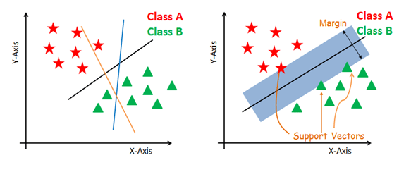
Points **outside the support vectors** are **100%** prediction accuracy.
Points **inside the support vectors** are **less 100%** prediction accuracy.

### Code:

from sklearn.svm import SVC

clf = SVC(kernel='linear', C=1.0, gamma=0.01)

clf.fit(X, y)

The bigger `C` (constrain), the more overfitting, the less points can be within the support vectors.

**Another definition of `C`**:
We use C (hyperparameter) to allow points within our margins ('on the street')
- Higher C = strong penalty. The more points we allow on the street, the bigger the hinge loss will become. When C is big enough, no point is even allowed within our margins. This is hard margin, and this can lead to overfitting
- Lower C = weak penalty. More points are allowed within the margins

The bigger `gamma`, the more curves the hyperlane has.

## Kernal Method
Still use a hyperplane to seperate classes, but project data points to $2^n$ higher dimension.

n = the original dimension.

### The Lagrange Multiplier
[Lagrange multiplier](https://en.wikipedia.org/wiki/Lagrange_multiplier) is a method for finding the extremum of a function with contraints. Consider the optimization problem:

*maximize* $f(x,y)$
*subject to*: $g(x, y) = 0$

<img src="https://cdn.kastatic.org/ka-perseus-images/98a7772076e49fa60eef3b3062a540ddc7130ad5.png" width="50%" />

<img src="https://upload.wikimedia.org/wikipedia/commons/f/fa/Lagrange_multiplier.png" width="30%" />

## GridSearchCV

gridsearch_models = GridSearchCV(clf, param_grid, cv=2, verbose=True, n_jobs=-1, scoring='accuracy')

best_model = gridsearch_models.best_estimator_

# no need to retrain because best_model is the result of the trained best model
# best_model.fit(X_train_flat, y_train_sample) 

predictions = best_model.predict(X_train_flat)

- `cv`: K-fold cross validation. Train k times with different set of training and validation data set.
- `scoring`: Balanced data set -> use accuracy; Unbalanced data set -> use f1 or roc_auc.

# Day 3
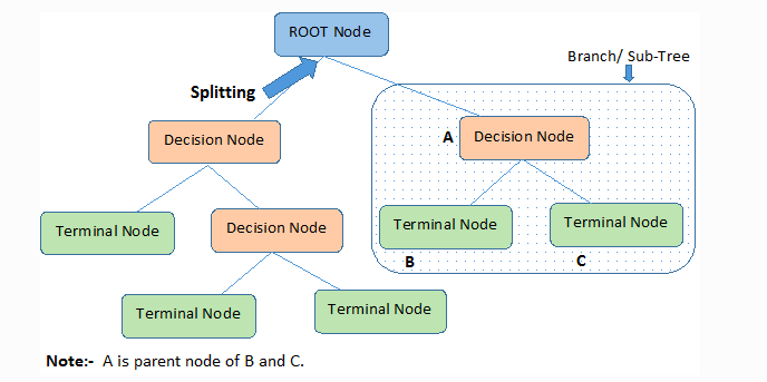
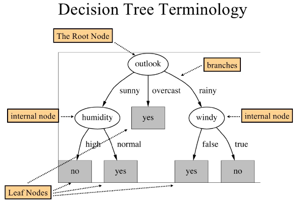
## Decision Tree
### Basic Definitions:


**Different kinds of Scoring**

### Gini Score
A measure of impurity.
Max = The splited group is mixed 50%
Min = No mix in the splited group
**Gini score is between 0 and 0.5**

Gini score is probability of each items in the group.

Each probability is squared to make sure Gini score

### How to select the feature to split:
Try different features and calculate Gini scores. The feature with the lowest Gini score will be chosen.

However, the feature with the lowest Gini score sometimes leads to more layers/nodes in the tree.

Decision tree treats **categorical and numerical** data in the **same** way.

Decistion tree tries **every single values** in the features to set the condition for the features. Finding circled numbers.

#### Steps:
1. Select feature to slit
2. Score the split: Gini scores of each group.
3. Get **weighted average** value of all Gini scores in all nodes.
4. Choose the lowest Gini score as the main feature to split.

### Can use multiple conditions/features to split at once, but it will lead to complexity conditions.

The splitting rule of Decision tree: Result of split must be 2 groups.

### Overfitting Tree:
Overfitting tree can produce **classes that only contain 1 data point**.

### Code

from sklearn.tree import DecisionTreeClassifier, DecisionTreeRegressor, plot_tree

clf = DecisionTreeClassifier(max_depth=3, criterion='gini', min_sample_leaf=5).fit(X_train, y_train)  # criterion = 'gini' or 'entropy'

# Draw decision tree graph
plt.figure(figsize=(20,10))
plot_tree(clf, filled=True, fontsize=14)
plt.show()

**max_depth** = Number of layers the tree can have.
**min_sample_leaf** = If number of records in a node is less than min_sample_leaf record => don't split.

### Results:
**Result of Decision Tree** algorithm is a **massive function** with a bunch of **if-else conditions** inside.

**Decision Tree vs Logistic Regression**

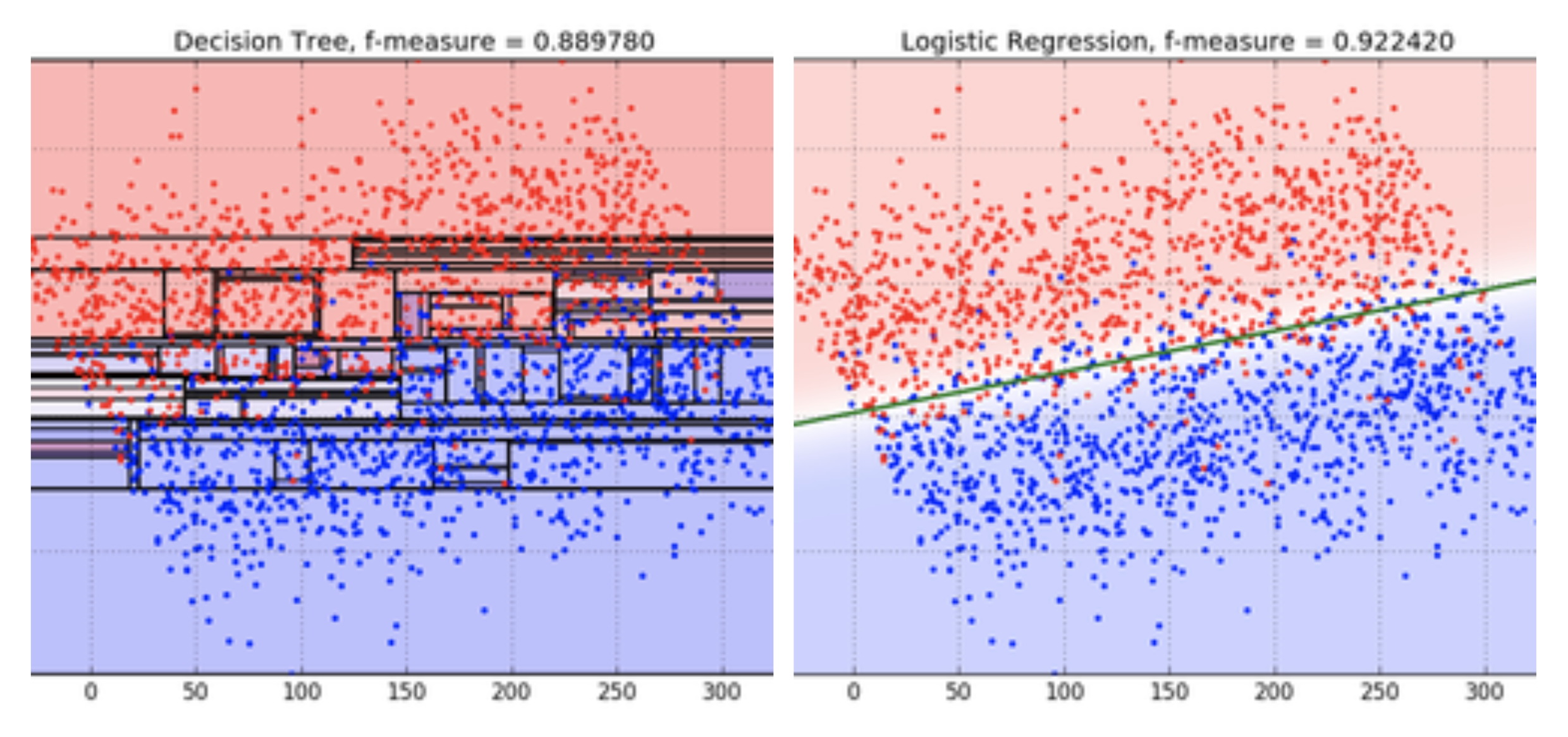
-> Should only use Decision Tree with complex shape data.

### Decision Tree for Regression:
#### Result:
Model prediection = Average of values in splitted groups.

Find the point to split that produces the smallest any regression metrics (MSE...).

## Bagging or Bootstrap:
Creating **samples** with the **same size** as the **original** data by **duplicating random data points** to **replace other data points**.
Then, use the samples to train models (1 sample - 1 model), then combine all of them or select all of the best ones.

### Random Forest:
Creating samples with random data points and **data features (columns)**.

**Different samples will create different trained model**, which can be very good at predict for that trained sample and may be overfitting.
However, when combining all of the trained models, the **overfitting/underfitting of the trained models will be cancelled eachother in the combined model**.

**Not throwing any model away**.

### Boosting

In boosting, the ensemble also consists of weak learners (e.g. Decision Tree). The key concept behind boosting is to **focus on training samples that are hard to classify**. In other words, **let the weak learners subsequently learn from misclassified training samples to improve the performance of the ensemble**.

Can throw away some models if its error is higher than a threshold.

**Other Boosting**:
- XGBoost is a boosting library with parallel, GPU, and distributed execution support.
- Gradient boosting.
- Microsoft's LightGBM and Yandex' CatBoost. Both of these libraries can match (and even outperform) XGBoost, under certain circumstances.

### AdaBoost

The algorithm assigns weights to all data points, samples the next training set based on the weights of the data points:

1. Initialize **all of the train set instance's weights equally**, so their sum equals 1.
2. Generate a **new set by sampling with replacement, according to the weights.**
3. **Train a weak learner** on the sampled set.
4. **Calculate its error** on the original train set.
5. **Add the weak learner to the ensemble** and **save its error rate**.
6. **Adjust the weights, increasing the weights of misclassified instances and decreasing the weights of correctly classified instances.**
7. Repeat from Step 2.
8. The weak learners are combined by voting. **Each learner's vote is weighted, according to its error rate**.

<img src="https://i.imgur.com/rWJy2jK.png"/>

## Comparison:

## Pipeline

Input of a pipeline must be a sklearn transformation Class.

**A sklearn transformation Class** must has **fit** and **transform** method (function).

In sklearn, method **fit_transform** executes 1 data type preparation and 2 methods **continuously**:
- **change data type to numpy array**
- **fit**: for preparation
- **transform**: for excecution from the output of preparation.

**Additional input** in sklearn transformation Class (each pipeline step) must be a **numpy array**.

**Output** of each sklearn transformation Class (each pipeline step) is a **numpy array**.

Example:

from sklearn.base import BaseEstimator, TransformerMixin

rooms_ix, bedrooms_ix, population_ix, households_ix = 3, 4, 5, 6

class CombinedAttributesAdder(BaseEstimator, TransformerMixin):
    def __init__(self):
        pass
    def fit(self, X, y=None):
        return self  # nothing else to do
    def transform(self, X):
        """Add new "columns" in an array (transformed from a dataframe).
        """
        rooms_per_household = X[:, rooms_ix] / X[:, households_ix]
        population_per_household = X[:, population_ix] / X[:, households_ix]
        bedrooms_per_room = X[:, bedrooms_ix] / X[:, rooms_ix]
        return np.c_[X, rooms_per_household, population_per_household,
                      bedrooms_per_room]

### SimpleImputer:
Scikit-Learn provides a handy class to take care of missing values: SimpleImputer

from sklearn.impute import SimpleImputer # this allow putting this part into a Pipeline

imputer = SimpleImputer(strategy="median")

# the median can only be computed on numerical attributes
housing_num = housing.drop("ocean_proximity", axis=1)
imputer.fit(housing_num)

### Categorical Encoding
Change string category to number.

#### OrdinalEncoder
Apply a **range of numbers** (0, 1, 2, 3...) to categories by sorting the categories **alphabetically** (by default), can customize the order of categories.
-> This will let to **biased** results: 1 category has **larger number** than other category.
This technique only works with pre-set (already known) order categories.

from sklearn.preprocessing import OrdinalEncoder # this allow putting this part into a Pipeline

housing_cat = housing[["ocean_proximity"]]
ordinal_encoder = OrdinalEncoder()
housing_cat_encoded = ordinal_encoder.fit_transform(housing_cat)

#### OneHotEncoder
Transform categories into **"vectors"** in a similar way to **pandas get_dummies**.

OneHotEncoder will create new columns for each category and delete the original categorical column.

from sklearn.preprocessing import OneHotEncoder # this allow putting this part into a Pipeline

cat_encoder = OneHotEncoder()
housing_cat_1hot = cat_encoder.fit_transform(housing_cat)
housing_cat_1hot
cat_encoder.categories_

## Split the data with the same distribution

housing["income_cat"] = pd.cut(housing["median_income"],
                               bins=[0., 1.5, 3.0, 4.5, 6., np.inf],
                               labels=[1, 2, 3, 4, 5])
                               
train_set, test_set = train_test_split(housing, test_size=0.2, random_state=42, stratify=housing['income_cat'])

## RandomizedSearchCV
Set ranges for hyperparameters, then RandomizedSearchCV will select randomly a number of sets to train the models.

from sklearn.model_selection import RandomizedSearchCV

# Day 4: Unsupervised Learning
## K-means
K-means put data points into clusters where the distance between data points and the central point of the clusters are the smallest.

Check out this [visualization](https://www.naftaliharris.com/blog/visualizing-k-means-clustering/) of the k-means algorithm.

**Expectation-Maximization**

In short, the expectation–maximization approach here consists of the following procedure:

1. Guess some cluster centers.
2. Step 2 - E-step: Assign each data point to the nearest cluster center.
3. Step 3 - M-step: Move the centroids to the center of their clusters.
4. Step 4: Keep repeating steps 2 and 3 until the centroid stop moving a lot at each iteration.


<img src="https://upload.wikimedia.org/wikipedia/commons/e/ea/K-means_convergence.gif">

## Hierarchical Clustering Algorithms
**No need to predefine number of cluster**.

### Agglomerative clustering (AGNES)
It works in a **bottom-up manner**.

The algorithm will define number of clusters itself by:
- Calculating the disctance of each data points;
- And group 2 data points that have the shortest distance as 1 group then repeat until there is no more new group or reach the desired number of groups.

### Divise Analysis (DIANA)
It works in a **top-down manner**.

## Principal Component Analysis (PCA)
This is only a technique to reduce number of features by creating new features (columns) from the original data set with projection rules.

PCA **reduces the dimensionality** of the data set, allowing **most of the variability** to be **explained** using **fewer** variables.

It is all about projecting high dimension data points into lower dimension where the variance of the data set is maximized.

**PCA is still reversable**, but **partial information will be lost**. However, PCA inverse will **make up data to cover the lost data**.

[Visualization](https://setosa.io/ev/principal-component-analysis/)

[PCA Calculation slides](https://docs.google.com/presentation/d/1nsWab3c_HpRAj3lXumUTTBhm9HVoisZvUlI6X0S2npU/edit#slide=id.p)

from sklearn.decomposition import PCA
pca = PCA(n_components=2)
# n_components: number of dimension to project on

pca.fit(X)

print(pca.components_)
print(pca.explained_variance_ratio_)

- `components_`: array, shape (n_components, n_features): Principal axes in feature space, representing the **directions of maximum variance** in the data. The components are sorted by explained_variance_.
- `explained_variance_ratio_`: array, shape (n_components,):
Percentage of variance explained by each of the selected components. The **percentage of the data set are kept (not losing)**.