---
tags: Kermadec Class, Machine Learning, Inferential Statistics, pivot, get_dummies, melt, mass change column names, Sort Day of Week, Sort Weekday, Distribution, Hypothesis, Significant Level (α), p-value
---

Machine Learning Week 4
=

# Day 1:
**[Slide](https://www.beautiful.ai/player/-MJMgHTDcwOk1RqzxoB1/FTMLE_41_Inference-Statistics)**
Inferential Statistics
||Descriptive Statistics | Inferential Statistics
|---|---|---
|**How to get the result**| Survey | Test
|**Purpose**|Describe a sample | Use result of that sample to test on population

Probability:
Independence vs Dependence

## Binomial Distribution: Binary outcome (head/tail coin)

Number of ways a desired result can happen:
Combination Formula (Number of Arrangement): `nCk`, n >= k

**Probability of each ways is dependent.**

The next "way" can't be the same as the previous "way".

Binomial Probability Formula:

**Example:** The ratio of boys to girls for babies born in Russia is 1.09 : 1

Boys / Girls = 1.09

Boys / Children = Boys / (Boys + Girls)


## Normal Distribution:
Continuous Probability


## Central Limit Theorem:
**Sufficiently large** random samples will be approximately well represeneted the population.

From the samples, we can calculate the means and standard deviation of the population.

## Hypothesis Testing:

A|B Testing

Hypothesis Testing will help conclude that the result of the sample is representative enough for the population.

### Null Hypothesis (H0) Opposite Alternative Hypothesis (H1)
**Null Hypothesis:** Nothing change, nothing happen. The current fact.
**Alternative Hypothesis:** Something change, something happen. What trying to be proved.

### Significant Level ($\alpha$):
The probability of rejecting the null hypothesis when it (the null hypothesis) is true (Type 1 error), aka **deny the truth**.

**The probability of allowing H0 to be wrong ~ Thresdhold.**

Example: In jury, the default state of Person is innocent until being proven guilty.

In business: standard $\alpha$ = 0.05 (5%)
In medical: standard $\alpha$ = 0.01 (1%)

***Guity = 1 = Positive
Innocent = 0 = Negative***


### Statistics Tests:
- **T-test**
- [One-sample T-test on scipy](https://docs.scipy.org/doc/scipy/reference/generated/scipy.stats.ttest_1samp.html)

***Example***: Orange juice business is booming. Nhan sets up a test by collecting sample sales of 10 random days. He wants to test if the average sale of orange juice can be more than 600 cups a day.

Sample values: `[587, 602, 627, 610, 619, 622, 605, 608, 596, 592]`

    import scipy # science python
    from scipy import stats

    # One-sample T-test
    
    sample = [587, 602, 627, 610, 619, 622, 605, 608, 596, 592]

    t, p = stats.ttest_1samp(a=sample, popmean=600)

    # popmean: Expected value in null hypothesis. If array_like, then it must have the same shape as a excluding the axis dimension.

- [Two sample T-test](https://docs.scipy.org/doc/scipy/reference/generated/scipy.stats.ttest_ind.html)

***Example***: Orange is not the only new black. Apple is also now an on-trend juice at Nhan's area. Nhan decides to survey 10 testers, who try both flavours and give a score to each on the scale of 1 to 10. He wants to see if there is any significant difference between the two flavor score.

The result is:

- Orange's Rating: `[1, 2, 2, 3, 3, 4, 4, 5, 5, 6]`
- Apple's Rating: `[1, 2, 4, 5, 5, 5, 6, 6, 7, 9]`

Can he draw the conclusion that the two flavors are different in term of taste rating?

    import scipy # science python
    from scipy import stats

    # One-sample T-test
    orange = [1, 2, 2, 3, 3, 4, 4, 5, 5, 6]
    apple = [1, 2, 4, 5, 5, 5, 6, 6, 7, 9]

    t, p = stats.ttest_ind(orange, apple)

- [**Z-test**](https://www.statsmodels.org/devel/generated/statsmodels.stats.weightstats.ztest.html)

Choose Z-test and T-test based on **sample size and population variance (mean)**
-> Most of the time we use T-test because we don't know about population unless there is a research before with a variance/mean result of a large sample. In this case, that large sample can be considered as population.

ANOVA
Chi-Square

### p_value:
**p_value** is the probability of getting type 1 error.

**The real probability of H0 is true.**

p_value return from `stats.ttest_1samp`: float or array; **Two-sided p-value**.
If H is 1 tail test (only larger or only smaller) -> p_value = p_value / 2

### Compare p_value with $\alpha$ to conclude:
p_value < $\alpha$ -> reject H0.
p_value >= $\alpha$ -> not enough eveidence to reject H0.


# Day 2
## Advanced Pandas

### Difference between df.groupby and pd.pivot_table

[pd.pivot_table](https://pandas.pydata.org/pandas-docs/stable/reference/api/pandas.pivot_table.html)
`pd.pivot_table` can fillna as well with option `fill_value`.

`pd.crosstab` same as pivot_table but for array types. pd.crosstab does not need input dataframe.

### get_dummies
[pd.get_dummies](https://pandas.pydata.org/pandas-docs/stable/reference/api/pandas.Series.str.get_dummies.html)

### melt
[pd.melt](https://pandas.pydata.org/docs/reference/api/pandas.melt.html)

Similar to Transpose, but can select certain columns to display at the same time.

### replace with nan value
df.column_name.replace('\xa0', value=np.nan, inplace=True)

**pd.replace**
- If **regex=False**, it only replace "to_replace" when the **whole value** of a cell equal to "to_replace".
- If **regex=True**, it will replace "to_replace" when the **cell contains** "to_replace".

### Mass Change Column Names:

df.columns = ['Maker','BarName','REF','ReviewDate','CocoaPercentage','Country','Rating','BeanType','BeanOrigin']

### Work with Geo things:
Work with dataframe with **geometry** column
`import geopandas as gpd`

Draw polygons based on **geometry** column
`import geoplot as gplt`

**Interactive chart/map:**
`import plotly.graph_objects as go`
This has pre-set polygons in the library.
No need to use custom **geometry** data, same as Google Studio Data Map.

# Day 3 Pandas Time Series

## Time Series Type:
Language is also a times series data.

Timestamp
Time intervals
Time periods
Time deltas or Duration

## Format Time:
strftime() and strptime()
https://docs.python.org/3/library/datetime.html#strftime-and-strptime-behavior

||strftime|strptime
|-|-|-|
Usage | Convert object to a string according to a given format | Parse a string into a datetime object given a corresponding format
Type of method | Instance method | Class method
Method of | date; datetime; time | datetime
Signature | strftime(format) | strptime(date_string, format)

## Time Index:

- For ***time stamps***, Pandas provides the ``Timestamp`` type. The associated Index structure is ``DatetimeIndex``.
- For ***time periods***, Pandas provides the ``Period`` type. The associated index structure is ``PeriodIndex``.
- For ***time deltas*** or ***durations***, Pandas provides the ``Timedelta`` type. The associated index structure is ``TimedeltaIndex``.

The most fundamental of these date/time objects are the **Timestamp** and **DatetimeIndex** objects. While these class objects can be invoked directly, it is more common to use the pd.to_datetime() function, which can parse a wide variety of formats.
* Passing **a single date** to `pd.to_datetime()` yields a **Timestamp**
* Passing **a series of dates** by default yields a **DatetimeIndex**.

### Time Index Slicing:
A Pandas series of time (DatetimeIndex) can do slicing:

## Generate Date Range:
`pd.daterange()` similar to `range()`
pd.daterange() has parameter (option) `freq`

| Code | Description | Code | Description |
|--------|---------------------|--------|----------------------|
| ``D`` | Calendar day | ``B`` | Business day |
| ``W`` | Weekly | | |
| ``M`` | Month end | ``BM`` | Business month end |
| ``Q`` | Quarter end | ``BQ`` | Business quarter end |
| ``A`` | Year end | ``BA`` | Business year end |
| ``H`` | Hours | ``BH`` | Business hours |
| ``T`` | Minutes | | |
| ``S`` | Seconds | | |
| ``L`` | Milliseonds | | |
| ``U`` | Microseconds | | |
| ``N`` | nanoseconds | | |

## Group By Time
- `df.resample()` similar to **df.groupby()** but can group by certain part of date (year or month or date... from a timestamp). Also **need** to define **an aggeration function**.
- `df.asfreq()` can group by certain part of date (year or month or date... from a timestamp) but only select the data on the group by time. Have built-in `df.fillna()` method.
_2004-12-31: The data of date 2004-12-31, not sum or mean._

### Sort Day of Week:
groupby(df.column.dayofweek)

## Shifting Data/Index by Time:
* `df.shift()` shifts the data
* `df.tshift()` shifts the index. In both cases, the shift is specified in multiples of the frequency.


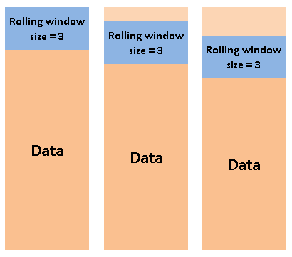
## Roling Window:
`df.rolling()`
Example: Average of 30 days around each day.

## Streamlit Starter Pack:
https://hackmd.io/VR6TV_4IQCKXc0IiG0UIQQ?view

# Day 4