---
tags: Kermadec Class, Machine Learning, Loss Function, MSE, Mean Squared Error, Gradient Descent, Polynomial Linear Regression, Confusion Matrix, Logistic Regression, Sentiment Analysis, Review Classification, Probability
---
Machine Learning Week 5
=
# Day 1:
## What is Machine Learning?
Mathematical model.
Without being explicitly programmed to provide output.
What is "without being explicitly programmed to do so"? And how?
T - P - E
Task - Performance measure - Experience
Example: Filter email
Mark spam email - Proportion of real spam vs identified spam - Emails
<img src="https://i.imgur.com/U3SAhRi.png" width="1000px"/>
## Supervised Learning:
- To learn a model from labeled training data.
- The learned model can make predictions about unseen data, data withouth label.
- **“Supervised”: the label/output of your training data is already known**.
### Supervised Learning Notaion:
The training data comes in pairs on $(x, y)$, where $x \in R^n$ is the input instance and y is label. The entire training data is:
$$
D = \{(x^{(1)}, y^{(1)}), \dots ,(x^{(m)}, y^{(m)})\} \subseteq R^n \times C
$$
where:
* $R^n$ is the n-dimensional feature space
* $x^{(i)}$ is the input vector of the $i^{th}$ sample - Data in other columns (beside the label column) of each row. 1 vector = 1 row of dataframe.
* $y^{(i)}$ is the label of the $i^{th}$ sample
* $C$ is the label space - Number of classes in the label, it can be infinity ($C=R$).
* $m$ is the number of samples in $D$ - Number of rows in dataset
**For the label space $C$:**
* When $C = \{0, 1\}$ or $C$ consists of two instances only, we have a **Binary Classification** problem. Eg. spam filtering, fraud detection.
* When $C = \{0, 1, \dots, K\}$ with $K > 2$, we have a **Multi-class classification** problem. Eg. face recognition, a person can be exactly one of $K$ identities.
* When $C=R$, we have a **Regression** problem. Eg. predict future temperature.
## Rules = Function $h$
<img src="https://i.imgur.com/nHOsIXv.png" width="1000px"/>
The data points $(x^{(i)}, y^{(i)})$ are drawn from some distribution $P(X, Y)$. Ultimately we would like to
- Learn a function $h$. $h$ is the function that the model will use.
- For a **new pair $(x, y) \sim P$, we have $h(x) \approx y$ with high probability.**
The feature vector $x^{(i)} = (x^{(i)}_1, x^{(i)}_2, \dots, x^{(i)}_n)$ consists of $n$ features describing the $i^{th}$ sample.
## Loss Function:
Linear Regression accuracy.
Mean Squared Error (MSE)

$$
\text{Mean Squared Error} = \frac{1}{m} \sum_{i=1}^{m}{(\hat{y}^{(i)} - y^{(i)})^2}
$$
```
def mse(y, y_hat):
return ((y_hat - y)**2).mean()
```
`y_hat` is the predicted value from linear regression.
`y` is the real value.
The central challenge in machine learning is that **the model must perform well on new, previously unseen input**.
## Overfitting and Underfitting
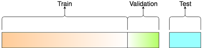
**Overfitting** if Accuracy with **Validation** data is way **more** than Accuracy with **Train** data.
Train: Doing exercise to get better, but if training too much, it will **remember the output** of each input, **not the pattern**.
**Underfitting** if Accuracy with **Validation** data is way **less** than Accuracy with **Train** data.
Overfitting and Underfitting are bad, it will lead to **bad prediction**.
## Probability:
Probability is only a translation of real life chances.
The **compliment** of $A$ is $A^C$, and $P(A^C) = 1 - P(A)$
**"compliment": opposite chances**
### Expected Value:
When performing a lot of tests, the expected value (outcome) will be equal to the mean value.
-> **Central Limit Theorem**
[Visualization](https://seeing-theory.brown.edu/probability-distributions/index.html)
### Variance Faster Calculation:
The **variance** measures the dispersion
$$
Var(X) = E[(X - E[X])^2]
$$

```
X1 = np.array([33,34,35,37,39])
var = np.mean(X1**2) - np.mean(X1)**2
```
[See theory through animation](https://seeing-theory.brown.edu/)
# Day 2
## Vector:
A vector represents the **magnitude** (length) and **direction** (arrow) of potential change to a point.
A line with direction, does **not depend on start/end points**.
Normal table -> transform to vectors to apply maths on the data.

3D
### Magnitude:
Magnitude: (length) of a vector:
Notation: Length of $\vec{v}$ = ||v||
`np.linalg.norm(v)`
Multiplication of a scalar and a vector:
Change vector length.
Negative scalar -> change direction.
### Unit Vectors:
**Unit vectors** are vectors of length 1, only care about direction, onlt length.
$\hat{i}$=(0,1) and $\hat{j}$=(1,0) are **the basis vectors** of $R^2$ (xy coordinate system).
That means **you can represent any vector in $R^2$ using i and j**
$$
\vec{v} = \begin{pmatrix} v_1 \\ v_2 \end{pmatrix}
= v_1.\begin{pmatrix} 1 \\ 0 \end{pmatrix} + v_2.\begin{pmatrix} 0 \\ 1 \end{pmatrix}
= v_1.\hat{i} + v_2.\hat{j}
$$
### Dot Product:
**Result of Dot product is always a scalar (1 number)**.
Different from **Hadamard product (Element-wise multiplication)**.
```
a = np.array([1,2,3])
b = np.array([4,5,6])
dot_product = 1*4 + 2*5 + 3*6
```
$$
\vec{a}.\vec{b} = \sum_{i}^{n}{a_ib_i} = ||a||.||b||.cos\phi
$$
`np.dot(my_rating,s1_rating)`


Dot product of $\vec{a}$ and $\vec{b}$ is
- **is positive** when they point at **similar** directions. Bigger = more similar.
- **equals 0** when they are perpendicular.
- **is negative** when they are at **dissimilar** directions. Smaller (more negative) = more dissimilar.
Dot product represents direction similarity of 2 vectors, but Dot product **is affected by vectors' length**.
**Example:**

s2_rating and s3_rating vectors are similar, but their Dot product is very small.
-> That is why we use **cosine similarity** to determine how similar it is between 2 vectors.
### Cosine Similarity:
From this you can calculate **similarity between 2 vectors** by calculating cosine of the angle $\phi$ between two vectors (known as **cosine similarity**).
Cosine similarity does not affect by vector magnitude (length).
$$
similarity(\vec{a},\vec{b}) = cos\phi = \frac{\sum_{i}^{n}{a_ib_i}}{||a||.||b||}
$$
`cosine_sim(my_rating,s2_rating)`

The resulting similarity is between -1 and 1, with
- −1: exactly opposite (pointing in the opposite direction)
- between -1 and 0: intermediate dissimilarity.
- 0: orthogonal, angel between 2 vectors are 90 degree.
- between 0 and 1: intermediate similarity
- 1: exactly the same (pointing in the same direction)

### Others:
**Magnitude (length)**: $||x||^2 = \vec{x}.\vec{x} $
**Commutative**: $\vec{x}.\vec{y} = \vec{y}.\vec{x}$
**Distributive**: $\vec{x}.(\vec{y} + \vec{z}) = \vec{x}.\vec{y} + \vec{x}.\vec{z}$
**Associative**: $\vec{x}.(a\vec{y}) = a(\vec{x}.\vec{y})$
**Vector projection:** $(\vec{x}.\vec{y})\frac{\vec{y}}{||y||^2}$

## Matrix:
Matrix is a collection of vectors.
**Review the Broadcasting**.
### Standard Normal Distribution:
Normalize each column (each column will have its own mean and std)
**Drag the mean to 0 and std = 1**.
**Tensorflow** always demand "Standard" matrix.
### Matrix Multiplication:
Matrix multiplication is a series of Dot product performing on each vector in the matrix.
For matrix multiplication, using '@' is prefered than np.dot.
https://numpy.org/doc/stable/reference/generated/numpy.dot.html
```
a = np.array([[1,2,3], [4,5,6]], dtype=np.float64) # we can specify dtype
b = np.array([[7,8], [9,10], [11, 12]], dtype=np.float64)
c = a @ b
```
**Do not FUCKING use this `c = np.dot(a, b)` for matrix Multiplication**.
It is confusing the Dot product between 2 vectors.
### System of Linear Equation:
\begin{cases}
ax_1 + bx_2 + cx_3 & = y_1 \\
dx_1 + ex_2 + fx_3 & = y_2 \\
gx_1 + hx_2 + ix_3 & = y_3
\end{cases}
$$
\Leftrightarrow
\underbrace{\begin{pmatrix}
a & b & c \\
d & e & f \\
g & h & i
\end{pmatrix}}_{M}
\underbrace{\begin{pmatrix} x_1 \\ x_2 \\ x_3 \end{pmatrix}}_{\vec{x}}
= \underbrace{\begin{pmatrix} y_1 \\ y_2 \\ y_3 \end{pmatrix}}_{\vec{y}}
$$
-> $\vec{y} = M\vec{x}$
## Derivative:
Derivative show the rate of changes of a function when the input change.
$$
f'(x) = \frac{df(x)}{dx} = \lim_{\Delta x \rightarrow 0} \Big( \frac{f(x + \Delta x) - f(x)}{\Delta x} \Big)
$$
The derivative measures the slope of the tangent line.
$y = ax + b$
a: slope
$a = (y2 - y1) / (x2 - x1)$
Slope shows the rate of changes.
Code
```
def df(x):
epsilon = 0.000001
return (f(x+epsilon) - f(x)) / epsilon
```
epsilon is the $\Delta x$
## Sigmoid Equation:
Sigmoid equation mimic the probability behavior (0-100%).
$\sigma (z) = \frac{1}{1 + e^{-z}}$

Being used in Machine Learning model a lot, but it is **not a perfect equation** because:
When z>>0 or z<<0 -> the slope of the tangent line = 0
## Partial Derivatives and Gradients:
**Gradient = Derivatives of a fuction with multiple input**.
How to solve it: find derivatives of **f and each x**, which is $\frac{\partial f}{\partial x_1}$.
`y = w @ X + b`
We consider the general case when $x \in R^n$, and, $f(x) = f(x_1, x_2, \dots, x_n)$. The generalization of the derivative to functions of serveral variables is the **gradient**.
$$
\nabla f = grad f = \frac{df}{dx} =
\Big[
\frac{\partial f}{\partial x_1} \
\frac{\partial f}{\partial x_2} \
\dots
\frac{\partial f}{\partial x_n}
\Big]
$$
<img src="https://i.imgur.com/b7zoo7n.png"/>
# Gradient Descent Algorithms:
**Purpose**: To get the minimum output of f(x).
$x = x - \alpha f'(x)$ ($\alpha$ is called the learning rate, which determines the step size). Let start with $\alpha=10^{-4}$
```
w = w - learning_rate*dw
b = b - learning_rate*db
```
The basic idea is **checking every point** on the Loss fuction to find the local minimum of the Loss function.
**Learning rate** will define **how long** the model will be traned.
The stipper the Loss function is, the smaller the Learning rate should be.
Example:
[Copy of 5.2c_Lab_Math_for_ML.ipynb](https://colab.research.google.com/drive/1uK5L0wCArW_fOO-mcP0QH7NsrIRXMB-A#scrollTo=Q-FiMdz9IZqe)
[Gradient Descent Animation](https://www.jeremyjordan.me/gradient-descent/)
# Day 3
## Linear Regression
- supervised machine learning algorithm.
- solves a **regression** problem. Predict **continuous output data**.
- **Input**: **vector** $x \in R^n$.
- **Output**: **scalar** $y \in R$.
- The value that our model predicts y is called $\hat{y}$, which is defined as:
$$
\hat{y} = w_1x_1 + w_2x_2 + \dots + w_nx_n + b = b + \sum^n{w_ix_i} = w^Tx + b
$$
where
<div align="center">
$w \in R^n$, and $b \in R$ are parameters.
$w$ is the vector of **coefficients**, also known as set of **weights**. $w^T$ is transpose of $w$.
$b$ is the **intercept**, also known as the **bias**.
</div>
$w$ and $b$ are the parameters of the function.
$x$ is the feature of the function.
<img src="https://i.imgur.com/b7zoo7n.png"/>
## Loss Function:
Using *minimizes the sum of squared errors (SSE) or mean squared error (MSE)**
$SSE = \sum_{i=1}^{n}(y - \hat y)^2$
$MSE = \frac{1}{n}SSE$
**Ordinary Least Squares (OLS) Linear Regression**
**Loss function** is **MSE or SSE**, which will draw a **curve line** (parabol shape).
### Gradient Descent:
**Gradient Descent** technique will try to **find the minimum output of Loss function** (MSE/SSE) by **changing the $w$ and $b$** in the Linear Regression function -> We will have a Linear Regression function with $w$ and $b$ closest to 0.
We want to minimize the **convex**, **continuous** and **differentiable** loss function $L(w, b)$:
1. Initialize $w^0$, $b^0$
2. Repeat until converge: $\begin{cases}
w^{t+1}_j = w^t_j - \alpha\frac{\partial L}{\partial w_j} & for\ j \in \{1, \dots, n\}\\
b^{t+1} = b^t - \alpha\frac{\partial L}{\partial b}
\end{cases}$
The Result $\frac{\partial L}{\partial w_j}$ in vectorization:
$$
\frac{\partial L}{\partial w} = \frac{2}{m} X^T . (\hat{y} - y)
$$
`dw = (2 / x_row) * (X.T @ (y_hat - y))`
The Result of $\frac{\partial L}{\partial b}$
$$
\frac{\partial L}{\partial b} = \frac{2}{m} \sum_{i=1}^{m}{(\hat{y}^{(i)} - y^{(i)})}
$$
`db = (2 / x_row) * np.sum((y_hat - y), keepdims=True)`

Code of how to train a Linear Regression:
```
from sklearn.linear_model import LinearRegression
from sklearn.metrics import mean_squared_error
X = df[['TV']]
y = df['Sales']
lr = LinearRegression()
lr.fit(X, y) # provide the best result already. coef_, intercept_ with the lowest Loss.
print(f'Weight: {lr.coef_}')
print(f'Bias: {lr.intercept_}')
print(f'MSE: {mean_squared_error(y, lr.predict(X))}')
plt.scatter(X, y, alpha=0.6)
plt.plot(X, lr.predict(X), c='r')
plt.show()
```
The smaller learning_rate is, the more accurate the result.
`learning_rate = 0.0000001`
The smaller learning_rate is, the bigger iterations needs to be.
`iterations = 1000000`
Standardize X (inputs) and y (labled) will help the training faster with **a bigger learning_rate** and **smaller iterations**.
```
# Standardization
# Skip this for now
x_mean = X.mean()
x_std = X.std()
X_scaled = (X - x_mean)/x_std
y_mean = y.mean()
y_std = y.std()
y_scaled = (y - y_mean)/y_std
# Training...
# If you use standardization
# scale w and b back to original unit
w_unscaled = w * (y_std/x_std)
b_unscaled = b * y_std + y_mean - (w_unscaled * x_mean)
print('Coef:', w_unscaled)
print('Intercept:', b_unscaled)
```
With simple loss function with only 1 local min.
At a certain iteration, the MSE will reach the min and stop changing.
## Normal Equations:
Faster way to solve Linear Regression.
Normal Equations (closed-form solution):
$w = (X^{T} X)^{-1} X^{T} y$
https://sebastianraschka.com/faq/docs/closed-form-vs-gd.html
## Polynomial Linear Regression:
Create curves in linear.
1 Curve = 1 Power.
More Curves -> The lower MSE on Training, but The more MSE on Validation.
## Overfitting vs Underfitting:
The ideal "fitting" is where the Error on Validation start to increase.
# Day 4
## Logistic Regression:
Logistic Regression is Linear Regression with the data labels are 0 or 1.
### Hyperplane:
A hyperplane is a subspace of its ambient space, and defined as:
$$
H = \{x: w^Tx + b = 0 \}
$$
* Examples, if a space is 3-dimensional then it's hyperplanes are 2-dimensional planes, while if the space is 2-dimensional, its hyperplanes are 1-dimensional lines.
* The hyperplane is perpendicular (vuông góc) to the vector $w$
$b$ is the bias term. Without $b$, the hyperplane that $w$ defines would always have to go though the origin.
Hyperplane is only used to classify binary classification (0, 1).

### Classifier:
A binary classifier with $y \in C = \{-1, +1 \}$ can be defined as:
$$
h(x) = sign(w^Tx + b) \\
y_i(w^Tx_i + b) > 0 \Leftrightarrow x_i \text{ is classified correctly} \\
$$
### Sigmoid:
Use Sigmoid function to give a probability of the accuracy on the classification result.
Result of $sign(w^Tx + b)$ are only +1 or -1.
Sigmoid of Z:
$$
\sigma (Z) = \frac{1}{1 + e^{-Z}} \\
Z = Xw + b \\
\hat{y} = \sigma(Z) = \sigma(Xw + b) = \frac{1}{1 + e^{-(Xw + b)}}
$$
Plug a linear regression in a Sigmoid function will give out the probability of prediction result.
### Cost Function:
**Binary cross entropy:**
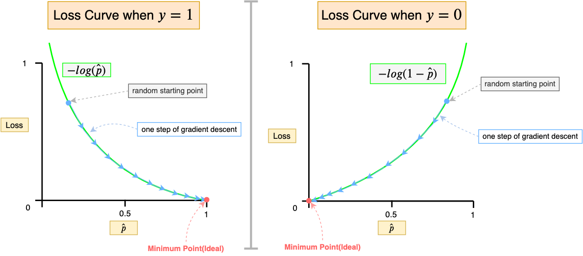
$$
Cost function = J(w, b) = -\frac{1}{m}\sum_{i=1}^m{ \Big( y^{(i)} log( \hat{y}^{(i)}) + (1-y^{(i)}) log(1 - \hat{y}^{(i)}) \Big)}
$$
`average_loss = -(np.mean(y * np.log(y_hat) + (1 - y) * np.log(1 - y_hat)))`
#### Why 1 Cost function has 2 ""graphs":
If y = 0:
$$
Cost function = J(w, b) = -\frac{1}{m}\sum_{i=1}^m{ \Big( 0 + (1-y^{(i)}) log(1 - \hat{y}^{(i)}) \Big)}
$$
If y = 1:
$$
Cost function = J(w, b) = -\frac{1}{m}\sum_{i=1}^m{ \Big( y^{(i)} log( \hat{y}^{(i)}) + (1-1) log(1 - \hat{y}^{(i)}) \Big)} \\
= -\frac{1}{m}\sum_{i=1}^m{ \Big( y^{(i)} log( \hat{y}^{(i)}) + 0 \Big)}
$$
### Gradient Desent:
**Still using Gradient Desent** with Binary cross entropy as Loss function.
**Forward Propagation:**
$$Z = Xw + b$$
$$\hat{y} = \sigma(Z) =\sigma(Xw + b) $$
$$J(w, b) = -\frac{1}{m}\sum_{i=1}^m{ \Big( y^{(i)} log( \hat{y}^{(i)}) + (1-y^{(i)}) log(1 - \hat{y}^{(i)}) \Big)}
$$
**and Backward**
$$ \frac{\partial J}{\partial w} = \frac{1}{m}X^T(\hat{y}-y)
$$
$$ \frac{\partial J}{\partial b} = \frac{1}{m} \sum_{i=1}^m (\hat{y}^{(i)}-y^{(i)})
$$
```
dw = (1 / x_row) * (X.T @ (y_hat - y))
db = (1 / x_row) * np.sum((y_hat - y), keepdims=True)
```
update_params
```
w = w - learning_rate*dw
b = b - learning_rate*db
```
### Output of Logistic Regression:
y_hat will be between 0 and 1, but we need y_hat must be 0 or 1.
=> Need to pick a threshold to round up/down the original y_hat.
### Code with Sklearn:
```
from sklearn.linear_model import LogisticRegression
from sklearn.metrics import confusion_matrix, accuracy_score
# Create Logistics Regression model from X and y
lg = LogisticRegression()
lg.fit(X, y)
predictions = lg.predict(X)
predictions_prob = lg.predict_proba(X)
# Show metrics
print("Accuracy score: %f" % accuracy_score(y, predictions))
# Show parameters
print('w = ', lg.coef_)
print('b = ', lg.intercept_)
```
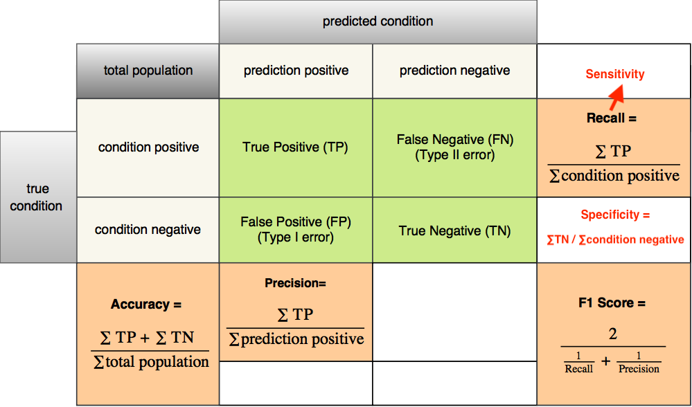
## Classification Model Evaluation - The Confusion Matrix
**Loss function in Logistic Regression is not as important as Confustion Matrix Metrics (Recall, Precision, Accuracy, F1 Score)**
```
from sklearn.metrics import confusion_matrix, accuracy_score, classification_report
from sklearn.metrics import log_loss
print("Accuracy score: %f" % accuracy_score(y_test, predictions))
print("Confusion Matrix:")
print(confusion_matrix(y_test, predictions))
print(classification_report(y_test, predictions))
print('Log loss:', log_loss(y_test, predictions)/len(y_test))
```
## Pickout Validation Sample:
```
from sklearn.model_selection import train_test_split
X_train, X_test, y_train, y_test = train_test_split(X, y, test_size=0.2, random_state=102)
```
# Day 5
## Sentiment Analysis with Logistic Regression
Sentiment: determine negative or positive tone of text content.
## Word to Vector:
### CountVectorizer with sklearn:
```
tweets = [
'This is amazing!',
'ML is the best, yes it is',
'I am not sure about how this is going to end...'
]
from sklearn.feature_extraction.text import CountVectorizer
# Define an object of CountVectorizer() fit and transfom your tweets into a 'bag'
count = CountVectorizer()
bag = count.fit_transform(tweets)
# Find in document of CountVectorizer a function that show us list of feature names
# sort alphabetically
count.get_feature_names()
```
**Word to number with CountVectorizer pattern**: Word count with the order of the vocab (bag of word), instead of the order of the input text.
**Example:**
['about', 'am', 'amazing', 'best', 'end', 'going', 'how', 'is', 'it', 'ml', 'not', 'sure', 'the', 'this', 'to', 'yes']
'This is amazing!': [0, 0, 1, 0, 0, 0, 0, 1, 0, 0, 0, 0, 0, 1, 0, 0]
'ML is the best, yes it is': [0, 0, 0, 1, 0, 0, 0, 2, 1, 1, 0, 0, 1, 0, 0, 1]
**Drawback:**
- No sentence order.
- Not supported acrynyms, only split by space.
There are better ways to transform word to numbers.
### Term Frequency-Inverse Document Frequency (TF-IDF):
**Term Frequency**: Appearances of 1 word in 1 text (1 document).
**Inverse Document Frequency**: Distinct appearances of 1 word in all of texts (all of documents). 1 word appear multiple times in 1 text is only counted as 1 for that text.
The **more appearances** of 1 word in all of the texts (documents), the **less important** the word is, the smaller the value in TfidfVectorizer.
sklearn use a **different method** to determine TF-IDF to deal with **log of 0**
Log of 0 appear when words in validation set do not appear in train set.
```
from sklearn.feature_extraction.text import TfidfVectorizer
tfidf = TfidfVectorizer(norm='l1', smooth_idf=False)
# Feed the tf-idf Vectorizer with tweets using fit_transform()
tfidf_vec = tfidf.fit_transform(tweets)
# Formatting the number to 2 digits after the decimal point
np.set_printoptions(precision=2)
# To print array in one line
np.set_printoptions(linewidth=np.inf)
```
### Removing stopwords:
```
import nltk
nltk.download('stopwords')
from nltk.corpus import stopwords
stop_words = stopwords.words('english')
['i',
'me',
'my',
'myself',
'we',
'our',
'ours',
'ourselves',
'you',
"you're",
"you've",
"you'll",
"you'd",
'your',
'yours',
'yourself',
'yourselves',
'he',
'him',
'his']
```
#### NLTK vs SpaCy vs Other libraries:
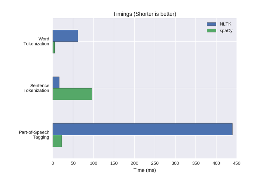
Read more: [Libraries of NLP in Python — NLTK vs. spaCy](https://medium.com/@akankshamalhotra24/introduction-to-libraries-of-nlp-in-python-nltk-vs-spacy-42d7b2f128f2#:~:text=NLTK%20is%20a%20string%20processing,and%20sentences%20are%20objects%20themselves.)
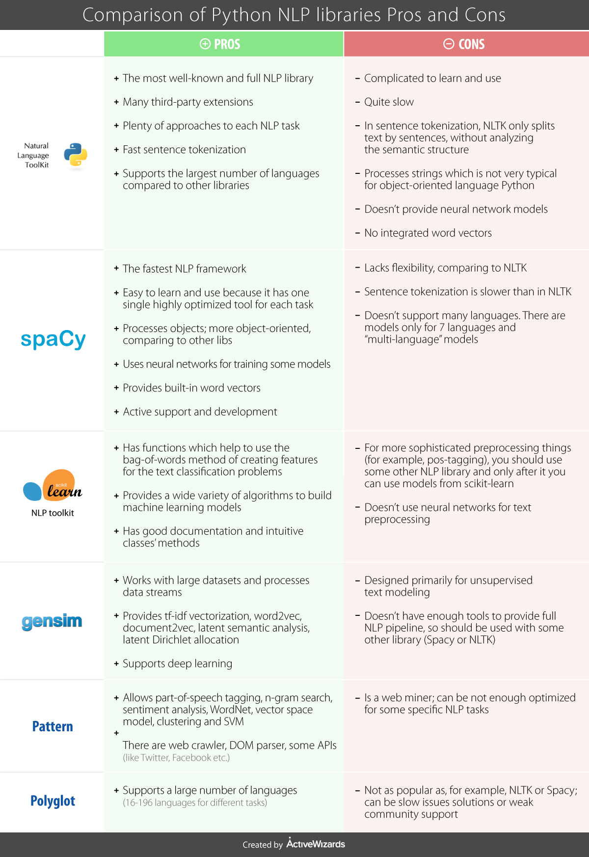
Read more: [Comparison of Top 6 Python NLP Libraries](https://medium.com/activewizards-machine-learning-company/comparison-of-top-6-python-nlp-libraries-c4ce160237eb)
### Removing special characters:
- HTML markup
- Save emoticons
- Remove any non-word character
### Stemming
Transform different form of a word into 1 word to minimize the noise.
**Example**:
Loving, loved, lovingly -> love
```
from nltk.stem import SnowballStemmer
porter = SnowballStemmer("english")
# Split a text into list of words and apply stemming technique
def tokenizer_stemmer(text):
return [stemmer.stem(word) for word in text.split()]
```
### Draw back of this vectorizing technique:
Taking too much consideration on the **distribution of words among the whole texts/documents**.
Only producing good result if **words distribution** of train set is similar to the test set.
 Sign in with Wallet
Connect another wallet
Sign in with Wallet
Connect another wallet