# [GDG TEAM 2] Amazon Electronics Customer Feedback
:::info
:bulb:This project revolutionizes how businesses understand customer feedback through advanced analytics and machine learning. Designed specifically for Amazon electronics product data, our system transforms raw customer reviews into actionable business intelligence, including:
:small_blue_diamond: Exploratory Data Analysis (EDA)
:small_blue_diamond: Customer Satisfaction Prediction using ML
:small_blue_diamond: Product Category Clustering
:small_blue_diamond: Review Sentiment Analysis using AI/DL
:small_blue_diamond: Recommendation System
:::
:::success
:information_source: Check our website for an interactive experience: [GDG Team 2](https://team2-amazon-gdg.vercel.app/)
The website tutorial can be found here: [Tutorial](https://drive.google.com/file/d/1SfrQ133PhjvsT3mR5t586bCiGah5yr3p/view?fbclid=IwY2xjawKf3xhleHRuA2FlbQIxMAABHtGUr3AhzpNcLQOwtkOyIyMxH_iByH8oZTluupq_ZetnXSTtn7Ega92p4b_6_aem_3h2IDz2PpWOLXmjyhSkfag)
:::
# 1. Data Preprocessing and Cleaning
:small_orange_diamond: Input: raw csv file `amazon.csv` contain the raw, unprocessed data which we will work on.
:small_orange_diamond: Output: cleanded csv file `amazon-cleaned.csv` contain the clean and formated data for further analysis in later steps.
## 1.1. Data transformation
- Drop the `discount_percentage` since can be calculated back from price and discounted_price.
- Several columns seems unnecessary for the following analysis were dropped: `product_link`, `img_link`, `user_name`.
- Convert price formats to numerical types, values that can not be converted will be assigned as `NaN`.
- Encode categorical variables such as category and user.
- Tokenize and clean review text for 2 columns (`review_title` and `review content`) including steps like remove hyperlinks, emojis, emoticons, puctuations, remove stopwords, lemmatization.
Before cleaning:
```tex!
Looks durable Charging is fine tooNo complains,Charging is really fast, good product.,Till now satisfied with the quality.,This is a good product . The charging speed is slower than the original iPhone cable,Good quality, would recommend,https://m.media-amazon.com/images/W/WEBP_402378-T1/images/I/81---F1ZgHL._SY88.jpg,Product had worked well till date and was having no issue.Cable is also sturdy enough...Have asked for replacement and company is doing the same...,Value for money
```
```tex!
durable charge fine toono complain charge fast good product satisfied quality good product charge speed slow original iphone cable good quality recommend
```
- Since each original observation are several reviews concatnated together to form a row, we split them back with `delimiter = ","`. This step, however will introduce unmatched columns between `user_id` and `review content` since review content have higher number of commas. This may happenned during the data crawl part which we have no control over.
## 1.2. Missing data
- After transformation, there is no missing data.
# 2. Exploratory Data Analysis (EDA)
:::info
**Analysis Objectives**
🔹 Understand the characteristics of product data and customer review behavior.
🔹 Explore the factors influencing:
* **Customer satisfaction**
* **Product popularity** (through `rating_count` and the number of reviews)
* **Discount effectiveness** (through `discount_percentage` and `discounted_price`)
:::
## 2.1. Data Overview
- Number of rows: $1446$.
- Number of columms: $10$.
- Key variables:
- `category`: Encoded using digital compression techniques $(1, 2, 3,...)$
- `discounted_price`: Price after discount, in INR (₹).
- `actual_price`: Original price before discount, in INR (₹).
- `rating`: Average customer rating (out of 5).
- `rating_count`: Number of customer ratings.
- `review_title`: Title of the customer review.
- `review_content`: Detailed content of the customer review.
## 2.2. Univariate analysis
### 2.2.1. Price distribution
- Actual_price ranges from 39.0 to 139,900.0
- Average price: 5,269.48
- Median: 1,639.00
- Standard deviation: 10,466.19
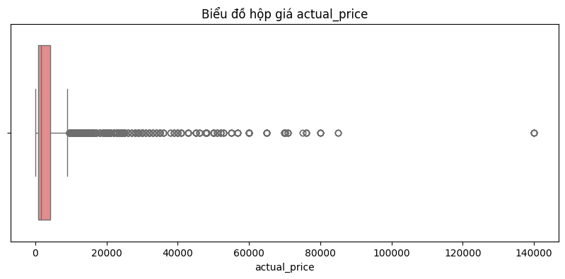
Comments:
:::info
The price distribution is very right-skewed, meaning that most of the products are in the low and middle price range (nearly 1.639), but there are a few very expensive products that extend the right tail of the distribution, causing the average price to increase significantly (5,269.48).
The median is much lower than the mean, indicating that most of the products are quite affordable, but a few very expensive products increase the average price significantly.
The very large standard deviation reflects a strong dispersion of prices, as there are many outliers that are very high compared to the rest of the data.
:::
### 2.2.2. Discount rate
$$\text{Discount Rate} = \frac{\text{actual_price} - \text{discounted_price}}{\text{actual_price}} \times 100\%
$$
.png)
- Average discount: 47.68%
- Discounts ranging from 30% to 70% are most common.
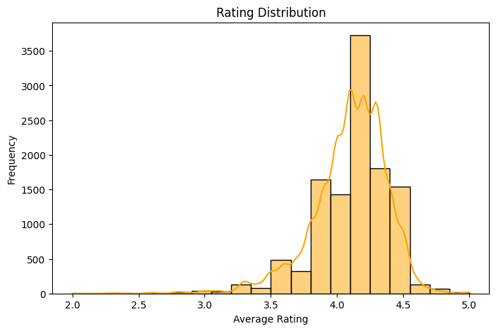
### 2.2.3. Rating
Approx. 76.03% of products have an average rating ≥ 4.0, indicating that most products are rated positively.
The most common rating is 4.1, suggesting a generally favorable perception across users.
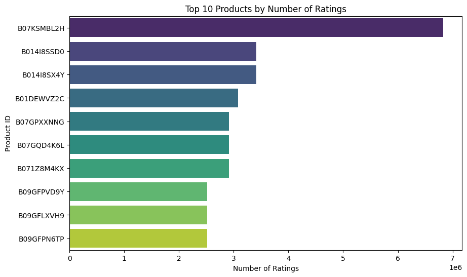
### 2.2.4. Identify the most popular products
## 2.3. Bivariate division
### 2.3.1. Discount vs. popular
| Metric | Correlation coefficient |
| -------- | -------- |
| discount_percentage vs rating_count | +0.42 |
A correlation coefficient of +0.42 between discount_percentage and rating_count suggests a moderate positive relationship.
**Interpretation:**
- As the discount percentage increases, the number of ratings tends to increase as well.
- This may indicate that products with higher discounts attract more buyers, which leads to more user engagement (i.e., reviews).
- However, the correlation is **not** very strong.
### 2.3.1. Rating vs. Rating count
Correlation coefficient between rating and rating_count: **0.10**
There is almost no meaningful linear association between the average rating of a product and how many reviews it receives.
## 2.4. Analyze the relationship between price, discount and rating
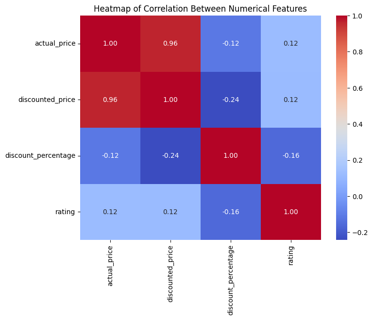
- Actual price and discounted price are highly correlated (0.96), as expected.
- Discount percentage has a small negative correlation with both prices, indicating that pricier products generally have lower discount rates.
- Rating is weakly positively correlated with prices, meaning higher-priced products tend to have slightly better ratings.
- Rating is weakly negatively correlated with discount percentage, suggesting that products with higher discounts may have slightly lower ratings.
Overall, price strongly relates to discounted price, but discount levels and ratings show only weak associations.
# 3. Customer Satisfaction Prediction
:::info
**Objective**
Build Machine Learning model for multi-class classification task to predict satisfaction based on selected features
:::
## 3.1. Classification model
:small_orange_diamond: Input: feature matrix **X** and label **y**
:small_orange_diamond: Output: trained models and performance metrics for each models
### 3.1.1 . Data preprocessing
- Create feature matrix **X**: the feature matrix is created by combining data from selected columns (`review_title`, `review_content`, `discount_percentage`, `category`, `rating`). With `review_title` and `review_content` are combined into `review_text`
- Create label **y**: the satisfaction is the target for the model to predict, this label is created by encoding process based on rating. The output is an array of label coresspoding for each data
- Implementaion: `encode_satisfaction(rating)`
- Encoding rule:
```python
def encode_satisfaction(rating):
if rating < 3:
return 0 # unsatisfied
elif rating < 4:
return 1 # neutral
else:
return 2 # satisfied
df['satisfaction'] = df['rating'].apply(encode_satisfaction)
```
- Remove rows containing null value to avoid training error.
- Comment: the dataset is highly imbalanced, with the label distribution is 73%, 26% and 1% for 3 class of lablel unsatisfied, neutral and satisfied, respectively. Based on this imbalanced, we need to have proper data sampling strategy to ultilize the training process.
### 3.1.2 Model Implementation
- Data sampling: we split the data into training and testing set, with 80-20 proportion for train and test set, using stratify technique based on label **y** to handle with imbalanced dataset.
- Implementation:
```python
# After cleaning duplicates and removing rating
X = df[['review_text', 'discount_percentage', 'category','rating']]
y = df['satisfaction']
# Split data with stratification
X_train, X_test, y_train, y_test = train_test_split(
X, y,
test_size=0.2,
stratify=y,
random_state=42)
```
- Data preprocessor: we further process the data using the following technique:
- `StandardScaler()`: normalized the numerical features (`rating`, `discount_percentage`) into the same value range.
- `OneHotEncoder()`: converted categorical feature (category) into binary vectors.
- `TfidfVectorizer()`: convert text data (`review_text`) into numerical features that machine learning models can understand.
- Implementation:
```python
preprocessor = ColumnTransformer(
transformers=[
('text', TfidfVectorizer(
max_features=500,
min_df=5,
max_df=0.7,
ngram_range=(1, 2),
stop_words='english'),
'review_text'),
('num', StandardScaler(), ['rating', 'discount_percentage']),
('cat', OneHotEncoder(max_categories=20,
handle_unknown='infrequent_if_exist'),
['category'])
],
remainder='drop)
```
- Model selection: `RandomForestClassifier` and `XGBClassifier` are used for this task, due to balanced training and inference ability to tracking back the most important feature sets.
- Parameters setting:
- Random Forest model:
```python
rf_model = RandomForestClassifier(
class_weight='balanced',
random_state=42)
```
- XGBoost model:
```python
xgb_model = XGBClassifier(
tree_method="hist",
use_label_encoder=False,
eval_metric='mlogloss',
random_state=42)
```
- Create ensemble model: to ensure robustness, generalization performance and reduce overfitting, we combine these 2 models into 1 ensemble model. The result will be the average result coming from the 2 models.
- Implementation:
```python
ensemble = VotingClassifier(
estimators=[
('random_forest', rf_model),
('xgboost', xgb_model)
],
voting='soft',
n_jobs=-1)
```
- Build the full pipeline: for clean and reusable code, we building a pipeline to put the ML process into a single object.
- Implementation:
```python
pipeline = Pipeline([
('preprocessor', preprocessor),
('classifier', ensemble)])
```
- Model training: to training the model, we called `fit` function from the `pipeline` and input feature matrix `X_train` and label `y_train`
- Implementation:
```python
# Train model
pipeline.fit(X_train, y_train)
```
## 3.3. Model Evaluation
We first evaluate models using Precision, Recall, and F1 Score for an accurate model examine. The result is reported in the table below.
| label | precision | recall | f1-score |
| ----- | --------- | ------ | -------- |
| 0 | 1 | 1 | 1 |
| 1 | 1 | 1 | 1 |
| 2 | 1 | 1 | 1 |
- Comment:
:::info
Although sampling data strategy has been adopted, the imbalanced between class labels affected a lot on this training result, led to an overfit model. This result can only be improved by re-collecting a more balanced dataset with the class proportion similar to each other.
:::
- Further evaluation:
- Confusion matrix: a detailed plot of confusion matrix shows how well our classification model is performing across three classes (0, 1, 2). The model has perfect classification on the test set with no off-diagonal errors (i.e., no misclassifications).

- Inference ability: using these tree-based model, we can also analyze the importance of each feature contributing to the result and conclude about what factors affect the most to customer satisfaction.


Note:
:::info
The plot above show multiple features but only some of them are real dataset features, due to data preprocessing for tree-based models. To have business decision, the analysis must select the real features to work on, for instance, `rating` or `discount_percentage` but not `working` or `receive` since they are not the real features.
:::
# 4. Product Category Clustering
:::info
**Objective**
Use unsupervised learning (e.g., K-Means, DBSCAN) to cluster products by price, discount, category, and user sentiment.
:::
## 4.1. K-Means clustering
### 4.1.1. Data Loading and Choosing Features
- Load the 'amazon-cleaned.csv' dataset (from the preprocessing notebook).
- Create back the column discounted percent
- We choose those numerical columns to perform clustering: num_cols = "actual_price", "discount_percent", "rating", "rating_count", "encode_review_rating".
- Remove duplicate rows since we only consider numerical features: number of rows from 11446 reduced to 1327.
### 4.1.2. Data Scaling:
- We use StandardScaler to transform the numerical columns into normal distribution with mean = 0 and variance = 1.
- Implementation
```
from sklearn.preprocessing import StandardScaler
scaler = StandardScaler()
X_train_scaled = scaler.fit_transform(X_train)
X_out_scaled = scaler.transform(X_out)
```
### 4.1.3. Principal Component Analysis
- We performed Pricipal Component Analysis (PCA) on the selected data frame to select the most importanct feature for the sole purpose of plotting.
- Plot pairwise plot between PC1, PC2 and PC3. We also plot a 3D scatter plot of those 3 PCs.
- Implementation
```
from sklearn.decomposition import PCA
pca = PCA()
pca.fit(X_train_scaled)
```
### 4.1.4. Apply K-Means
- We use KMeans() model from sklearn to perform K-Means clutering

- By using Elbow Method and analyse the Silhouette Score, we decided to choose the number of cluster, k = 5 as the optimal choice.
- 
- After labeling the dataset using model.predict, we scattered plot the first 3 leading PCs with their respective class (cluster). Result show that all clusters are well separated.
### 4.1.5. Evaluate Model
We calculated the following metrics:
- Silhouette Score (0.384): This indicate potential overlap between features
- Davies-Bouldin Index (0.842): This indicate moderate separation between clutsers.
- Calinski-Harabasz Index = 735.991
### 4.1.6. Analyse each cluster
- We calculated the mean for each cluster and for global to derive intuition.
| Cluster Mean | `actual_price` | `discount_percent` | `rating` | `rating_count` | `encode_review_raing` |
| :------------- | :------------- | :----------------- | :------- | :------------- | :-------------------- |
| Global | $5469.63$ | $0.529$ | $4.09$ | $18260.71$ | $1.745$ |
| Cluster 0 | $3098.50$ | $0.385$ | $4.21$ | $13799.78$ | $2.000$ |
| Cluster 1 | $3044.80$ | $0.480$ | $3.70$ | $8559.44$ | $0.997$ |
| Cluster 2 | $3800.16$ | $0.757$ | $4.24$ | $14282.31$ | $2.000$ |
| Cluster 3 | $2557.55$ | $0.489$ | $4.19$ | $246115.09$ | $1.970$ |
| Cluster 4 | $44233.07$ | $0.626$ | $4.25$ | $11314.44$ | $1.972$ |
- Cluster 0: Affordable, well-rated products with low discounts, suggesting good value or brand loyalty despite fewer average reviews.
- Cluster 1: Mid-priced items with normal discounts but very low ratings and review counts, indicating poor performance or limited customer appeal.
- Cluster 2: Mid-priced products with very high discounts achieve good ratings, suggesting sales are largely driven by the perceived value from markdowns.
- Cluster 3: Low-priced, highly-rated items with extremely high review counts, marking them as very popular, mass-market products.
- Cluster 4: High-priced, highly-rated premium items offered with significant discounts, likely appealing to a niche market despite fewer reviews.
## 4.2. DBSCAN
We perform identical step of Data Loading, Retain Numerical Features, Scale Data using ```StandardScaler()```, Applying PCA just like in K-Means clustering.
### 4.2.1. Apply DBSCAN
- The `DBSCAN` model from `sklearn.cluster` was used to perform density-based clustering on the scaled data (`X_train_scaled`).
* Parameter Tuning:
* To determine an appropriate `eps` (epsilon) value, the k-distance graph method was employed.
* Based on the "elbow" point in the k-distance graph, `eps` was chosen as 1.8.
* `min_samples` was set to 8.

* After applying DBSCAN with these parameters:
* Number of clusters found (excluding noise): 2
* Number of noise points (outliers): 4
* Below is the plot of 3 leading PCs with labels.

### 4.2.2. Model Evaluation
```
- Silhouette Score (DBSCAN): 0.600
- Davies-Bouldin Index (DBSCAN): 0.940
- Calinski-Harabasz Index (DBSCAN): 499.933
```
### 4.2.3. Analyse each cluster
| Metric Group | `actual_price` | `discounted_price` | `rating` | `encode_review_raing` |
| :---------------------- | :------------- | :----------------- | :------- | :-------------------- |
| Global Mean | $5525.44$ | $3201.33$ | $4.09$ | $1.737$ |
| Cluster -1 Mean (Noise) | $65598.50$ | $41446.75$ | $3.68$ | $1.250$ |
| Cluster 0 Mean | $6105.24$ | $3580.68$ | $4.23$ | $2.000$ |
| Cluster 1 Mean | $3150.50$ | $1660.40$ | $3.70$ | $1.000$ |
- Cluster -1 (Noise): extremely high-priced outlier products with lower-than-average ratings, setting them apart due to their distinct price points.
- Cluster 0: good quality, slightly above-average priced products that are consistently well-rated by customers.
- Cluster 1: more affordable, budget-friendly products that tend to receive lower ratings and less positive reviews.
## 4.3 Compare the results of K-Means and
K-Means was ultimately the better option over DBSCAN for this project due to the following reasons.
- **More cluster defined**: K-Means identify 5 clusters providing a more detailed breakdown of product categories, while DSCAN only form 2 clusters.
- **More insights**: The 5 segments from K-Means offered more diverse and directly interpretable profiles (e.g., "Mass-market popular," "Premium with discounts"), which is more beneficial for understanding varied market dynamics and tailoring strategies.
# 5. Review Sentiment Analysis
:::info
**Objective**
To further analyze the customer satisfaction, we leverage both traditional NLP and Deep Learning model to perform the customer sentiment analysis based on the `review_content`.
:::
## 5.1. Review classification
In this part, we apply traditional NLP (TF-IDF + ML classifiers) and Deep Learning models (BERT, RoBERTa) to classify reviews as Positive, Negative, or Neutral.
:small_orange_diamond: Input: A review text from customer
:small_orange_diamond: Output: Sentiment class of the review (`negative`, `neutral`, `positive`)
### 5.1.1. Traditional NLP
#### 5.1.1.1. Data Preprocessing
- Sentiment label: we obtained the sentiment label by mapping value from `satisfaction` feature column created at the previous model.
- Implementation:
```python
df['sentiment'] = df['satisfaction'].map({0: 'negative', 1:'neutral', 2: 'positive'})
```
- Distribution of sentiment classes: we obtain the same result as the above preprocessing result, with the imbalanced between the class of sentiment, where the amount of positive review dominated the amount of neutral and negative review.

#### 5.1.1.2. Model Implementation
- Data sampling: we construct the feature matrix **X** based on `review_content` and label **y** based on `sentiment` column above to create a matrix for training. We then split the data and sampling using the same methodolody as part 3 - Customer Satisfaction Prediction.
- Data preprocessing: using TF-IDF method to convert text into numerical vectors for ML model training. We only keep the top 5000 most frequent terms to reduce dimensionality.
- Implementation:
```python
tfidf = TfidfVectorizer(max_features=5000)
X_train_tfidf = tfidf.fit_transform(X_train)
X_test_tfidf = tfidf.transform(X_test)
```
- Model training and Prediction: after preprocessing the data, we input them into a class of supervised ML model - Logistic Regression and Support Vector Machine (SVM). The goal is to train a class of model which has the ability to predict the `sentiment` label base on the `review_content`
- Logistic Regression:
```python
lr = LogisticRegression()
lr.fit(X_train_tfidf, y_train)
lr_pred = lr.predict(X_test_tfidf)
```
- Support Vector Machine:
```python
svm = SVC()
svm.fit(X_train_tfidf, y_train)
svm_pred = svm.predict(X_test_tfidf)
```
#### 5.1.1.3. Model Evaluation
We evaluate the model across 4 different metrics: Accuracy, Precision, Recall and F1-Score. The result are reported in the plot below for a better overview as well as comparision between models.

- Comment: In overall, both model can predict the desire sentiment label with high evaluation metrics anf SVM produced slightly higher results across 4 metrics than Logistic Regression. This can be due to the learning ability of SVM since it can model the hyperplanes to separate the dataset, which then dealing with non-linear relationship better than Logistic Regression, where the relationship is assume to follow the logistic function at the beginning.
### 5.1.2. Deep Learning model
#### 5.1.2.1. Data Preprocessing
We first define the custome dataset class to wraps the `review_text` and `sentiment` label into a PyTorch-compatible dataset format for the Trainer.
- Implementation:
```python
class SentimentDataset(Dataset):
def __init__(self, texts, labels, tokenizer, max_len):
self.texts = texts
self.labels = labels
self.tokenizer = tokenizer
self.max_len = max_len
# Convert string labels to integers
self.label2id = {label: idx for idx, label in enumerate(sorted(set(labels)))}
self.labels = [self.label2id[label] for label in labels]
def __len__(self):
return len(self.texts)
def __getitem__(self, idx):
text = str(self.texts[idx])
label = self.labels[idx]
encoding = self.tokenizer.encode_plus(
text,
add_special_tokens=True,
max_length=self.max_len,
return_token_type_ids=False,
padding='max_length',
truncation=True,
return_attention_mask=True,
return_tensors='pt',
)
return {
'input_ids': encoding['input_ids'].squeeze(0),
'attention_mask':encoding['attention_mask'].squeeze(0),
'labels': torch.tensor(label, dtype=torch.long)}
```
- In `__init__`: Converts string labels ("positive", "negative") to integers using a dictionary.
- In `__getitem__`: Returns a dictionary with:
- `input_ids`: token IDs.
- `attention_mask`: tells model which tokens are real vs. padding.
- `labels`: integer label.
#### 5.1.2.2. Model Implementation and Training
- Model class: we first implement a full pipeline for DistilBERT. This pipeline then can be used to implement similar model such as BERT.
- Initialization: we first initialize tokenizer, model and prepare the dataset for the training process.
- Implementation:
```python
# Initialize tokenizer and model
tokenizer = DistilBertTokenizer.from_pretrained('distilbert-base-uncased')
# Initialize DistilBERT model
model = DistilBertForSequenceClassification.from_pretrained('distilbert-base-uncased', num_labels=len(set(y_train)))
# Prepare datasets
train_dataset = SentimentDataset(X_train, y_train, tokenizer, max_len=128)
test_dataset = SentimentDataset(X_test, y_test, tokenizer, max_len=128)
```
- Parameters setting: to training the model, we need to set up some parameters first.
- Implementation:
```python
training_args = TrainingArguments(
output_dir='/content/drive/MyDrive/Colab Notebooks/distilBert_results',
num_train_epochs=3,
per_device_train_batch_size=16,
per_device_eval_batch_size=16,
warmup_steps=500,
weight_decay=0.01,
logging_dir='/content/drive/MyDrive/Colab Notebooks/distilBert_logs',
eval_strategy='epoch',
save_strategy='epoch',
load_best_model_at_end=True,
)
```
- Model training: to training the model, we first initialize the `Trainer` with model and parameters setting above. Then we called the `train` function to training.
- Implementation:
```python
# Trainer init
trainer = Trainer(
model=model,
args=training_args,
train_dataset=train_dataset,
eval_dataset=test_dataset,
)
# Train
trainer.train()
```
#### 5.1.2.3. Model Evaluation
We first evaluate models using Precision, Recall, and F1 Score for an accurate model examine. The result is reported in the table below.
| label | precision | recall | f1-score |
| -------- | -------- | -------- | -------- |
| 0 | 1 | 0.88 | 0.93 |
| 1 | 1 | 0.99 | 1 |
| 2 | 1 | 1 | 1 |
- Comment: comparing to the traditional NLP model and ML models, we can observe the model is now less overfitting and provide a more generalized result.
- Further evaluation:
- Confusion matrix: a detail confusion matrix for the model can be found below.

- ROC curve: for a classifiction model, a ROC curve can be an useful metric to measure how well our model separate the data and perform predition compares to a random model. As the result, our DistilBERT model outperform random model in all classes of sentiment labels.

#### 5.1.2.4. Model Testing
Based on the trained model, we can then doing further testing. In this part we will try to input a review text from a customer and check if it can predict the sentiment label of the text correctly.
- Implementation: we first calling the `model` and the `tokenizer`, the set the model to `eval` mode and define a `predict_sentiment` function to perform testing the model.
```python
model = DistilBertForSequenceClassification.from_pretrained('/content/drive/MyDrive/Colab Notebooks/sentiment_model/distilBERT')
tokenizer = DistilBertTokenizer.from_pretrained('/content/drive/MyDrive/Colab Notebooks/sentiment_model/distilBERT')
# Set model to eval mode
model.eval()
# Load label2id and reverse it to get id2label
with open('/content/drive/MyDrive/Colab Notebooks/sentiment_model/distilBERT/label2id.json', 'r') as f:
label2id = json.load(f)
# Create id2label, ensuring keys are integers
id2label = {int(v): k for k, v in label2id.items()}
# Inference function
def predict_sentiment(text):
inputs = tokenizer(text, return_tensors="pt", padding=True, truncation=True, max_length=128)
with torch.no_grad():
outputs = model(**inputs)
probs = torch.nn.functional.softmax(outputs.logits, dim=1)
predicted_id = torch.argmax(probs, dim=1).item()
predicted_label = id2label[predicted_id]
return predicted_label, probs.squeeze().tolist()
```
- Testing: the model can return correctly the sentiment label for the review text as well as the coressponding probability values for each sentiment class. We can observed that the probalility of positive sentiment (number 2) is the highest compare to the other sentiment labels.
```python
text = "This is a good product with many functions."
label, probs = predict_sentiment(text)
print(f"Predicted label: {label}")
print(f"Probabilities: {probs}")
```
```
Predicted label: positive
Probabilities: [0.010573343373835087, 0.023851269856095314, 0.9655753970146179]
```
- BERT implementation: using the same above pipeline, the detailed implementation for BERT can be found on the Github link.
## 5.1. Customer review summarization
To perform customer review summarization task, we using the pre-trained BART model, due to the limitation in the dataset, where the summarization information is unavailable in the provided dataset, we cannot perform training based on this dataset.
:small_orange_diamond: Input: A long review text from customer.
:small_orange_diamond: Output: A shorter and summarize version of the review text.
- Model implementation: we first imported the `BartTokenizer` and `BartForConditionalGeneration` model for the BART architecture, then loading the `pipeline` from `transformers` which wraps all steps (tokenization, model inference, decoding). Finally we input a sentence and calling the pipeline to perform summarization task.
```python
from transformers import BartTokenizer, BartForConditionalGeneration
from transformers import pipeline
tokenizer = BartTokenizer.from_pretrained("facebook/bart-large-cnn")
model = BartForConditionalGeneration.from_pretrained("facebook/bart-large-cnn")
summarizer = pipeline("summarization", model="facebook/bart-large-cnn")
review_text = "I recently purchased this wireless Bluetooth speaker and overall, I’m pretty happy with it. The sound quality is excellent—clear highs and decent bass for the size. It’s compact and easy to carry around, which is perfect for my outdoor trips. The battery life lasts about 8 hours on a full charge, which meets my expectations.However, the delivery took longer than promised, arriving almost a week late. The packaging was a bit damaged, but thankfully the product inside was unharmed. Also, I had some trouble connecting it to my phone at first, but after restarting both devices it worked fine.For the price, I think it offers good value. I would recommend it to anyone looking for a portable speaker but be prepared for possible delivery delays."
summary = summarizer(review_text, max_length=100, min_length=30, do_sample=False)
print(summary[0]['summary_text'])
```
- Output result: after perform summarization, we obtained a text summarize from the input with shorter length and a concise content.
```
The sound quality is excellent and the battery life lasts about 8 hours on a full charge. The delivery took longer than promised, arriving almost a week late. I would recommend it to anyone looking for a portable speaker.
```
# 6. Recommendation System
## 6.1. Overview
:::info
**Objective**
The recommendation system is implemented as a key feature in the User Emulator tab, providing sellers with intelligent product suggestions based on various algorithms. The system is designed to help sellers understand customer preferences and improve their product offerings.
:::
Comment:
:::warning
We have trouble at two 2 .csv for web service and .json for webpage. So decide to get recommedation by using name of .json file that user click on webpage + .csv to store in database. When query we chunking file in web service storage to process data. When done it auto remove. This can cause to performance, long time respone or out of CPU
:::
## 6.2. Implementation Details
### 6.2.1. Frontend Implementation
- **User Interface:**
- Dropdown menu for selecting recommendation methods
- Input field for specifying number of recommendations (Top N)
- Grid display of recommended products
- Loading state indicator during API calls
- Pagination support for cluster-based recommendations
- **Features:**
- Real-time recommendation updates
- Visual display of product information
- Direct links to Amazon product pages
- Responsive grid layout for product cards
### 6.2.2. Backend Implementation
#### a) API Endpoints
```python
@app.route('/recommend', methods=['POST'])
def create_remmcommend():
query = request.args.get('method')
product_id = request.args.get('product_id')
top_n = request.args.get('top')
url = request.args.get('url')
```
#### b) Recommendation Algorithms
1. **Cosine Similarity**
- Implementation: `get_product_recommendations()`
- Features:
- Text-based similarity using TF-IDF
- Combines multiple product attributes:
- Product name
- Product description
- Category
- Review titles
- Review content
- Returns similarity scores for ranking
2. **Content-Based Filtering**
- Implementation: `get_user_based_recommendations()`
- Features:
- User behavior analysis
- Rating pattern matching
- Normalized similarity scoring
- Considers user rating history
3. **K-means Clustering**
- Implementation: `get_product_cluster()`
- Features:
- Pre-computed clusters stored in JSON
- Efficient product grouping
- Pagination support
- Cluster-based similarity
-
Comment:
:::warning
I have trouble with this because different data struture, respone. So at this time i use fix data that already cluster for using can get recommend. This route bring serveral problem i wish i have more time to fix this.
:::
### 6.2.3. Data Processing
- Price cleaning and normalization
- Text preprocessing for similarity calculation
- Rating normalization
- JSON response formatting
## 6.3. Technical Details
### 6.3.1. Dependencies
- pandas: Data manipulation
- numpy: Numerical operations
- scikit-learn: TF-IDF and similarity calculations
- Flask: API endpoints
- Supabase: Data storage
### 6.3.2. Performance Optimizations
- Cached cluster data
- Efficient data structures for user-product matrices
- Pagination for large result sets
- Error handling and validation
## 6.4. Usage Examples
### 6.4.1. Cosine Similarity
```python
recommendations = get_product_recommendations(
product_id='B07JW9H4J1',
csv_url='https://example.com/products.csv',
top_n=5
)
```
### 6.4.2. Content-Based Filtering
```python
recommendations = get_user_based_recommendations(
product_id='B07JW9H4J1',
csv_url='https://example.com/products.csv',
top_n=5
)
```
### 6.4.3. K-means Clustering
```python
recommendations = get_product_cluster(
product_id='B07JW9H4J1',
page=1,
page_size=10
)
```
## 6.5. Future Improvements
:::warning
1. Implement collaborative filtering
2. Add real-time cluster updates
3. Enhance similarity calculations
4. Add more recommendation metrics
5. Implement A/B testing supportinfo
:::
# 7. Interactive Dashboard
## 7.1. Overview
:::info
**Objective**
The dashboard is designed to serve data analysts and sellers, helping them visualize and analyze Amazon product data effectively. The interface is built with an intuitive approach, featuring tables, lists, and interactive tools arranged logically.
:::
## 7.2. Techincal + Structure
| | Stack | Host & DeployDeploy |
| -------- | -------- | -------- |
| Frontend | Vite, React, TypeScripts, React Router DOM | Vercel |
| Backend | Flask, FastAPI | Render, Modal |
| Database | PostgresSQL | Supabase |
| CSS & Component | TailwindCSS, Shadcn, Lucide React, Chart.js | |
:::info
The dashboard is divided into 3 main tabs:
:::
- Home
- Upload object
- Select object
- Product
- Notification
- Update user reviews realtime
- Realtime sentiment
- Product Performance
- Card Overview
- Search bar
- Filter select
- Table of products
- Customer Sentiment
- Analyze all reviews of the product
- Pricing & Discount
- Filter select
- Draw chart
- Draw plot
- Insights
- User Emulator
- Customer feedback
- Post the review
- Get recommend list
## 7.3. Feature Details
### Optimization
:::success
- To avoid Supabase rate limits and optimize performance, the ProductData provider is wrapped around all components. When data queries are needed, components call the provider to get the list
- All buttons with event handlers that send API requests use useState to disable them, preventing spam
:::
### 7.3.1. Home Tab

#### a) Data Upload and Processing
**Frontend:**
- Uses React hooks (`useState`, `useRef`) to manage file and input states
- File upload interface with "Upload new object" button and selected file name display
- Event handling through `handleFileChange` and `handleUpload`
**Backend:**
- API endpoint: `https://team2-amazon-gdg.onrender.com/convert`
- CSV file processing and conversion to JSON format
- JSON data storage in Supabase
#### b) Data List Display
**Frontend:**
- Uses `JsonFileList` service to fetch file list from Supabase table object .eq('json')
- Displays list with information:
- Index number
- File name
- Creation time (UTC format)
- Interaction: Click on file to navigate to Product tab with corresponding data
**Backend:**
- Data storage on Supabase
- Data URL: `https://wblqskhiwsfjvxqhnpqg.supabase.co/storage/v1/object/public/`
### 7.3.2. Product Tab

:::info
- Tablist for navigation to different functions:
- Product Performance
- Customer Sentiment
- Price & Discount
- Insights
:::
#### a) Data Analysis and Visualization
Comment:
:::warning
For display category and subcatgory by spliting | in product_category it bring me many time fixing, because algorithm, logic to display category level. Category level can affect every componnet in this page so maintaine this not easy. I use heriachy pattern do to design fucntion, use many states, list object to store category, really nightmare.
:::
**Frontend:**
- Main interface:
- Product search bar by name or ID
- Category filter with hierarchical structure
- Product table with detailed information
- "Load More" button for additional products
- Filtering and sorting features:
- Filter by category (Category/Subcategory)
- Sort by:
- Rating (ascending/descending)
- Number of reviews (ascending/descending)
- Price (ascending/descending)
- Visual charts:
- Bar Chart: Product rating distribution
- Pie Chart: Discount level distribution
- Price-Rating correlation chart
- Draw Plot: Chunking images returned from API according to corresponding data type
**Backend:**
- Product data processing:
- Basic information:
- Product ID
- Product name
- Category
- Original and discounted prices
- Discount percentage
- Review information:
- Rating (1-5 stars)
- Number of reviews
- Review content
- User information:
- User ID
- Username
- Review title and content
- Category hierarchy processing:
- Automatic category structure analysis
- Support for multiple category levels
- Product count by category
#### b) Review Sentiment Analysis
- Sentiment analysis model integration:
- Using DistilBERT model
- Real-time analysis
- Visual result display
- Interactive features:
- View review details
- Sentiment analysis per review
- Overall sentiment statistics
#### c) Interaction and Navigation
- Navigation to User Emulator for reviews
- Interaction with charts and data tables
- Responsive design for various screen sizes
### 7.3.3. User Emulator Tab

- **Frontend**
- For sellers wanting to build their own platform, a page is created where they can operate like on Amazon, view previous buyer reviews, post product reviews, and receive product recommendations
- Recommendation methods:
- Cosine similarity
- Content-based filtering
- Kmeans Cluster
- **Backend**
- Route `/recommend` accepts parameters `product_id`, `method`, etc.
## 7.4. Futher Improvement
- Middleware, JWT
- Open API document for developer
- Add authencation with Auth Provider `Google`, `Facebook`, `Github`
- Acess realtime with data from Amazon Seller API
- Improve web service for better responning process
- Clean code
- Create custom hook for easy maintain
- Restyling for better UI/UX
- Use more ico/svg for visualize
- Query database not use `select(*)`
- Realtime every component
- Microservices
- Role for management : adminstrator , partner, seller, ...
- Export to PDF
- Deepdive into report, use LLMs for function processing language and understanding context
 Sign in with Wallet
Connect another wallet
Sign in with Wallet
Connect another wallet