# AVL Trees

###### tags: `dsa`, `trees`

:::section{.introduction}
## Introduction
AVL (Adelson-Velsky and Landis) Tree is a self-balancing binary search tree that can perform certain operations in logarithmic time. It exhibits height-balancing property by associating each node of the tree with a balance factor and making sure that it stays between -1 and 1 by performing certain tree rotations. This property prevents the Binary Search Tree from getting skewed, thereby achieving a minimal height tree that provides logarithmic time complexity for some major operations such as searching.
:::

:::section{.scope}
## Scope of article
- This article provides an overview of AVL Trees data structure, its need, and its application in computer science.
- The article covers the various concepts related to AVL Trees and their implementation in C++ and Java.

:::

:::section{.main}
In our fast-paced daily lives, we make use of a lot of different data structures and algorithms without even noticing them. For example, consider a scenario that you wish to call someone from your contact list that contains a ton of data. For this, you need to find the phone number of that individual by using a searching process. This is internally implemented using specific data structures and uses particular algorithms to provide you with the best results in an efficient manner. This is required as the faster the search, the more convenience you get, and the faster you can connect with other people.

With time, this searching process was gradually improved by implementing and developing new data structures that eradicate or reduce the limitations of the previously used methods. One such data structure is AVL Trees. It was developed to reduce the limitations of the searching process implemented using a non-linear data structure known as Binary Search Trees.

Now, you may ask what exactly was the limitation and how AVL Trees overcome it, providing us with a better searching process in terms of efficiency. For this, let’s take a look at the Binary Search Trees (BSTs) search process, what are the limitations in this process and how the AVL Trees overcome them.
:::

::::::section{.main}
## Searching using Binary Search Trees
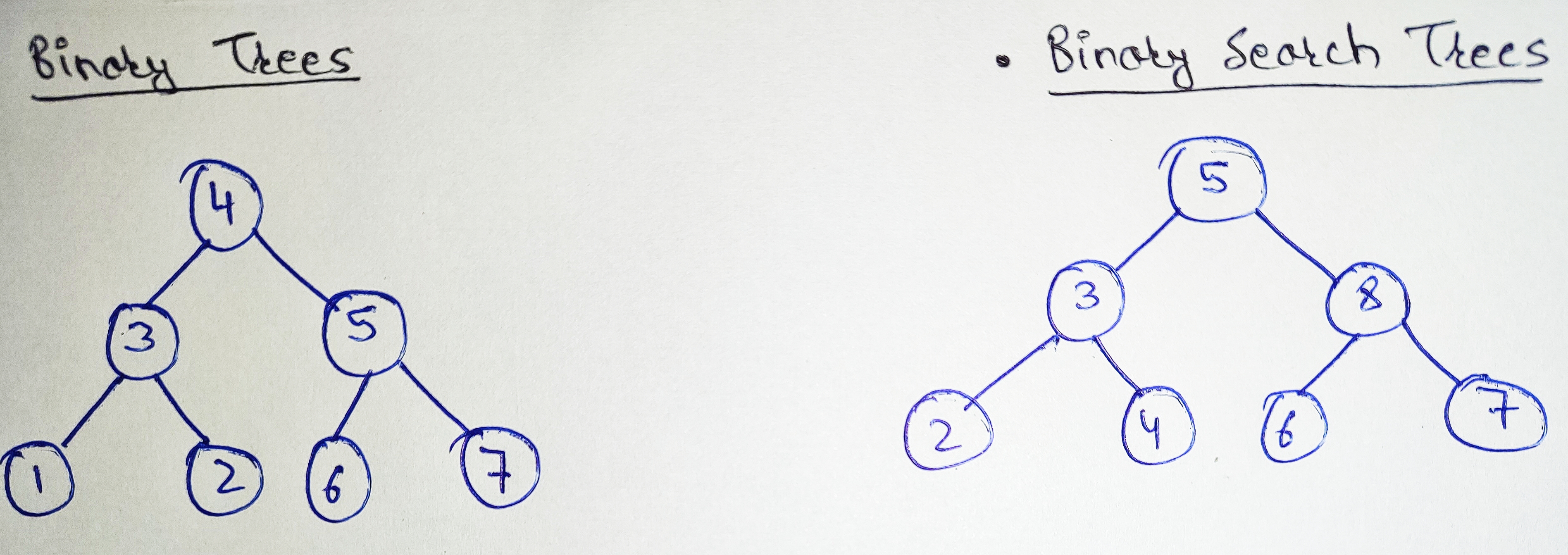
A Tree is a non-linear and hierarchical data structure that consists of a root node (the topmost node of the tree) and each node can have some number of children nodes. It represents an actual hierarchical tree structure such as your Family Tree. Now, a special case of trees is the Binary Trees i.e., trees in which every node has at most two children.

Furthermore, there exist [Binary Search Trees](https://en.wikipedia.org/wiki/Binary_search_tree) that are a special type of binary trees in which all the elements in the left subtree of a node are smaller than that node whereas all the elements in the right subtree are greater in value **(BST Rule)**.

:::section{.graphics}
:::

In the above example, you can notice that all the nodes of the Binary Search Tree follow the BST rule i.e., for all the nodes their left subtrees have lesser values while the right subtrees have greater values.

Binary Search Trees are useful in searching an element from a constantly updating data stream or in finding an element when a combination of search and update operations are being performed on a dataset.

Here, upon each updation in the data stream, the element is inserted in the BST and the search is performed based on the query provided. In BSTs, to find an element we start with the root node and check whether the given element is greater than the root node or not if it’s greater we continue searching in the right subtree otherwise we look in the left subtree. This process is continued until we find a node having the same value as that of the given query value, or we reach the leaf node of the tree i.e., the element is not present in the tree. In either case, the depth or the height of the tree (the number of edges on the longest path from the root node to a leaf node) defines the time complexity of the search operation.

Let’s understand this effect of height on the searching operation in BSTs with an example:

:::section{.sub-section}
### **Case 1: Unbalanced BST**

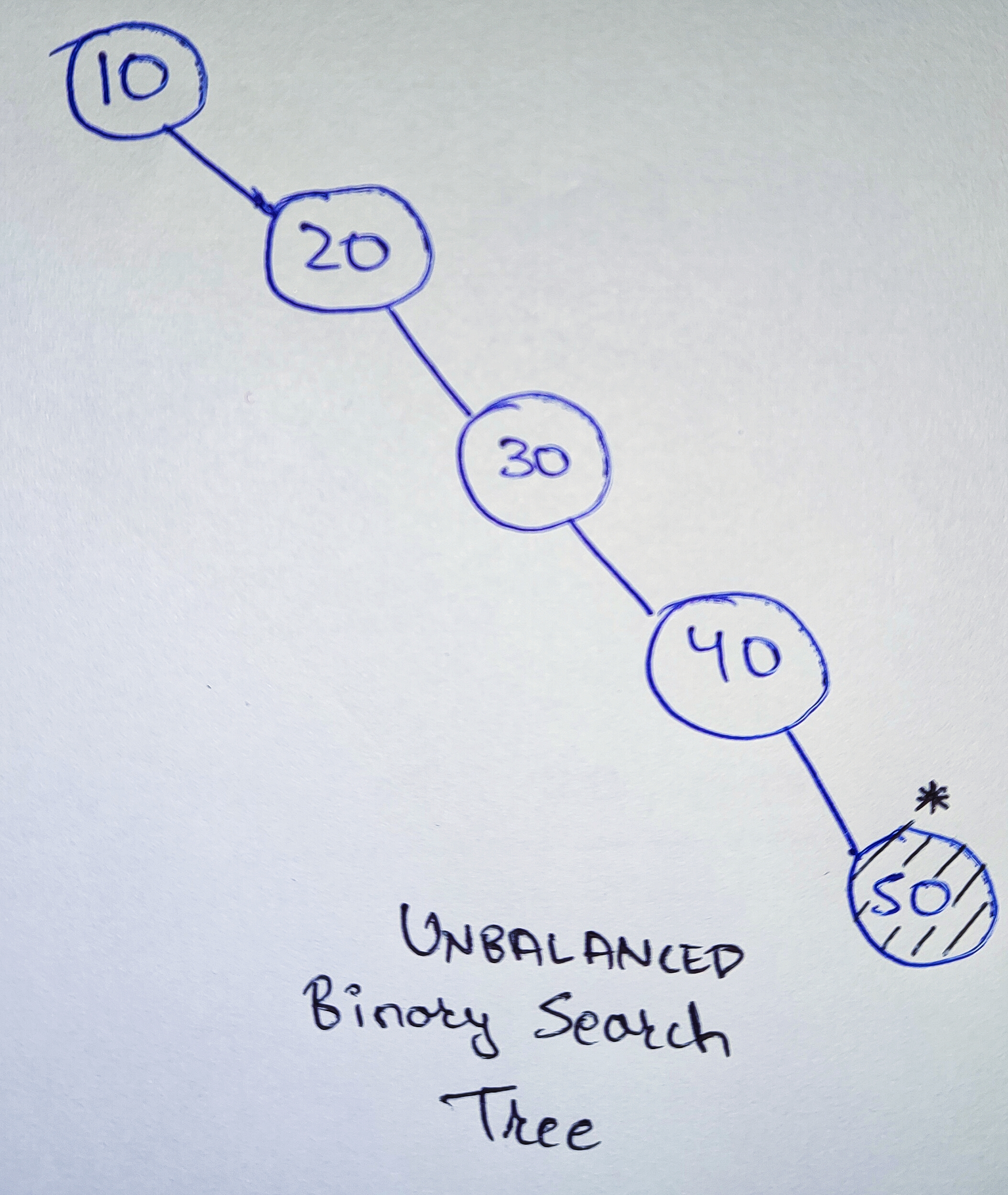
Consider a sorted array **A** having elements `[10, 20, 30, 40, 50]`. Now, when we create a BST for this array, all the elements will be inserted in the right subtree as all are having greater value than the previous element i.e., the BST becomes skewed or unbalanced (for a given node, one subtree is significantly larger than its sibling subtree) and will look like this:

:::section{.graphics}
:::

Now, if we wish to search whether the element `50` is present in this BST or not, we will have to traverse all the elements present in the BST as `50` is present at the deepest level of the tree. Also, there is no left subtree to traverse at each level. Hence, instead of reducing the number of checks at each level, we are just searching the element in **linear time** i.e., `O(n)`, where `n` is the total number of nodes present in the BST.
:::

:::section{.sub-section}
### **Case 2: Balanced BST**

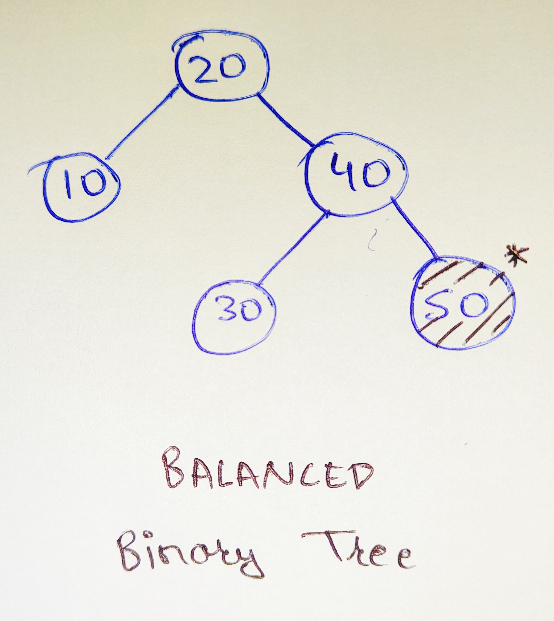
Now, consider another example in which the same elements are inserted in a different order such as `[20, 10, 40, 30, 50]`. In this case, when we create a BST using this order, it will attain minimal height and will look like this:

:::section{.graphics}
:::

Now, on searching the element `50` in this tree we are reducing the number of comparisons as in each step we are neglecting the left subtrees at each level i.e., we are reducing the check operations by half at each level. Hence, in this case, when the tree is not skewed, the process of searching takes **logarithmic time** i.e., `O (log n)` where `n` is the total number of nodes present in the tree.
:::

:::section{.main}
In the above example we can observe that when the tree was skewed in the First case, it attained the maximum height i.e., `O (n)` which is the same as the time complexity for the search operation in this case. Also, in the second case when the tree attained minimal height i.e., `O (log n)`, the search operation took logarithmic time. Hence, we can say that the height or the depth of the tree somewhat determines the time complexity of the BST.

Now, you may wonder that for the same elements we can have two Binary Search Trees having drastically different heights and search times. Hence, there must be a way to control the height of the BST such that we always achieve logarithmic search time complexity irrespective of the order of the elements. This can be achieved by checking when the Binary Search Tree starts becoming skewed **(Balancing Criteria)** and performing certain operations to limit this skewness. In this way, we can control the height of the tree and achieve a logarithmic time complexity for almost all the operations. This is exactly where AVL Trees come into action!!!
:::

:::section{.highlights}
**Highlights:**
1. BSTs are binary trees in which all elements in the left subtree of a node are smaller while the elements in the right subtree are larger than that node.
1. BSTs are useful to perform searches on dynamic datasets.
1. As the operations performed using BSTs always start from the root and traverse down the tree, the time complexity of BSTs depends upon the height of the tree.
1. BSTs can be skewed (unbalanced) or balanced depending upon the order of insertion of the elements.
1. Balanced BSTs provide logarithmic time complexity because of their optimal height.

:::
::::::

:::section{.main}
## What is an AVL Tree?

[AVL Tree](https://en.wikipedia.org/wiki/AVL_tree), named after its inventors Adelson-Velsky and Landis is a special variation of Binary Search Tree which exhibits self-balancing property i.e., AVL Trees automatically attain the minimal possible height of the tree after the execution of any operation. The AVL Trees implement the self-balancing property by attaching extra information known as the balance factor to each node of the tree, then verifying that the balance factor for all the nodes of the tree follows certain criteria **(Balancing Criteria)** upon the execution of any operation that affects the height of the tree, and finally applying certain **Tree Rotations** to maintain this criterion of height-balancing.

The Criterion of height balancing is a principle that determines whether a Binary Search Tree is unbalanced (skewed) or not. It states that:

:::section{.tip}
A Binary Search Tree is considered to be balanced if any two sibling subtrees present in the tree don’t differ in height by more than one level i.e., the difference between the height of the left subtree and the height of the right subtree for all the nodes of the tree should not exceed unity. If it exceeds unity, then the tree is known as an unbalanced tree.
:::

Since skewed or unbalanced BSTs provide inefficient search operations, AVL Trees prevent unbalancing by defining what we call a balance factor for each node. Let's look at what exactly is this balance factor.

:::section{.highlights}
**Highlights:**
1. AVL Trees were developed to achieve logarithmic time complexity in BSTs irrespective of the order in which the elements were inserted.
1. AVL Tree implemented a Balancing Criteria (For all nodes, the subtrees’ height difference should be at most 1) to overcome the limitations of BST.
1. It maintains its height by performing rotations whenever the balance factor of a node violates the Balancing Criteria. As a result, it has self-balancing properties.
1. It exists as a balanced BST at all times, providing logarithmic time complexity for operations such as searching.

:::
:::

:::section{.main}
## Balance Factor

The balance factor in AVL Trees is an additional value associated with each node of the tree that represents the height difference between the left and the right sub-trees of a given node. The balance factor of a given node can be represented as:

balance_factor = (Height of Left sub-tree) - (Height of right sub-tree)

Or mathematically speaking,

$$
bf = h_l - h_r
$$

where ***bf*** is the balance factor of a given node in the tree, ***hl*** represents the height of the left subtree, and ***hr*** represents the height of the right subtree.

:::section{.graphics}
:::

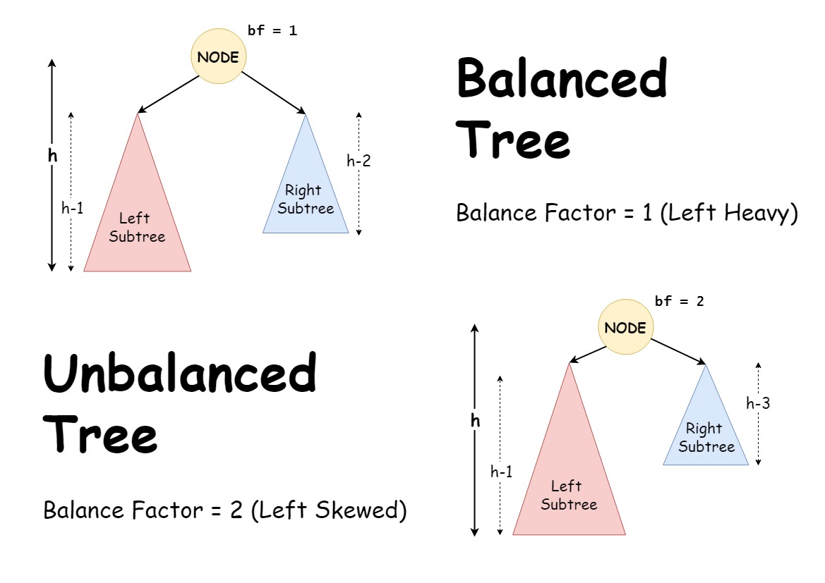
In the balanced tree example of the above illustration, we can observe that the height of the left subtree `(h-1)` is one greater than the height of the right subtree `(h-2)` of the highlighted node i.e., the given node is left-heavy having the balance factor of positive unity. Since the balance factor of the node follows the Balancing Criteria (height difference should be at most unity), the given tree example is considered as a balanced tree.

Now, in the unbalanced tree example, we can observe that the tree is left-skewed i.e., the height of the left subtree is much greater than that on the right subtree. This is clearly an unbalanced tree as it is highly skewed. This is also indicated by the balance factor of the node as it doesn’t follow the Balancing Criteria.

Hence, AVL Trees make use of the balance factor to check whether a given node is left-heavy (height of left sub-tree is one greater than that of right sub-tree), balanced, or right-heavy (height of right sub-tree is one greater than that of left sub-tree). Hence, using the balance factor, we can find an unbalanced node in the tree and can locate where the height-affecting operation was performed that caused the imbalance of the tree.

:::section{.tip}
**NOTE -** Since the leaf nodes don't contain any subtrees, the balance factor for all the leaf nodes present in the Binary Search Tree is equal to `0`.
:::

Upon the execution of any height-affecting operation on the tree, if the magnitude of the balance factor of a given node exceeds unity, the specified node is said to be unbalanced as per the Balancing Criteria. This condition can be mathematically represented with the help of the given equation:

$$
bf = (h_l – h_r), s.t. bf ∈ [-1, 0, 1]
$$

Or

$$
|bf| = |h_l - h_r| ≤ 1
$$

Here, the above equation indicates that the balance factor of any given node can only take the value of -1, 0, and 1 for a height-balanced Binary Search Tree. To maintain this criterion for all the nodes, AVL Trees take use of certain **Tree Rotations** that are discussed later in this article.

:::section{.highlights}
**Highlights:**
1. Balance Factor represents the height difference between the left and the right sub-trees for a given node.
1. For leaf nodes, the balance factor is 0.
1. AVL balance criteria: |bf| ≤ 1 for all nodes.
1. Balance factor indicates whether a node is left heavy, right heavy, or balanced.

:::
:::

::::::section{.main}
## AVL Tree Rotation

As discussed earlier, the AVL Trees make use of the balance factor to check whether a given node is left-heavy (height of left sub-tree is one greater than that of right sub-tree), balanced, or right-heavy (height of right sub-tree is one greater than that of left sub-tree). If any node is unbalanced, it performs certain **Tree Rotations** to re-balance the tree.

:::section{.tip}
**Tree Rotations:** It is the process of changing the structure of the tree by moving smaller subtrees down and larger subtrees up, without interfering with the order of the elements.
:::

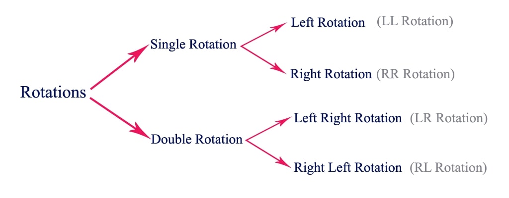
If the balance factor of any node doesn't follow the AVL Balancing criterion, the AVL Trees make use of 4 different types of Tree rotations to re-balance themselves. These rotations are classified based on the node imbalance cured by them i.e., a specific rotation is applied to counter the change that occurred in the balance factor of a node making it unbalanced.

These rotations include:

:::section{.graphics}
:::

Now, let's look at all the tree rotations and understand how they can be used to balance the tree and make it follow the AVL balance criterion.

:::section{.sub-section}
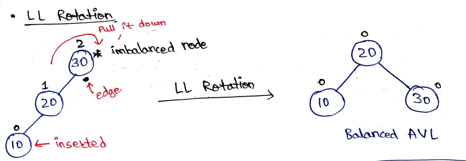
### 1. LL Rotation

It is a type of single rotation that is performed when the tree gets unbalanced, upon insertion of a node into the left subtree of the left child of the imbalance node i.e., upon **Left-Left (LL) insertion**. This imbalance indicates that the tree is heavy on the left side. Hence, a **right rotation (or clockwise rotation)** is applied such that this left heaviness imbalance is countered and the tree becomes a balanced tree. Let’s understand this process using an example:

Consider, a case when we wish to create a BST using elements 30, 20, and 10. Now, since these elements are given in a sorted order, the BST so formed is a left-skewed tree as shown below:

:::section{.graphics}
:::

This is confirmed after calculating the balance factor of all the nodes present in the tree. As you can observe, when we insert element `10` in the tree, the root node becomes imbalanced `(balance factor = 2)` because the tree becomes left-skewed upon this operation. Also, notice that element `10` is inserted as a left child in the left subtree of the imbalanced node (here, the root node of the tree). Hence, this is the case of **L-L insertion** and we will have to perform a certain operation to counter-act this left skewness.

Now, imagine a weighing scale in which we only have 5 kg on the left plate and nothing on the right plate. This is the case of left heavy since there is nothing on the right plate to balance the weight present in the left plate. Now, to balance this scale we can just add some weight to the right plate. Hence, to balance the weight on one side we try to increase the weight on the other side. In the case of trees, instead of adding a new node (weight) on the lighter side, we try to rotate the structure of the tree around a pivot point thereby shifting the nodes from the heavier side to the lighter side.

In our example, we have extra weight on the left subtree (LL insertion) therefore we will perform right rotation or clockwise rotation on the imbalanced node to transfer this node on the right side to retrieve a balanced tree i.e., we will pull the imbalanced node down by rotating the tree in a clockwise direction along the edge of the imbalanced or in this case, the root node.
:::

:::section{.sub-section}
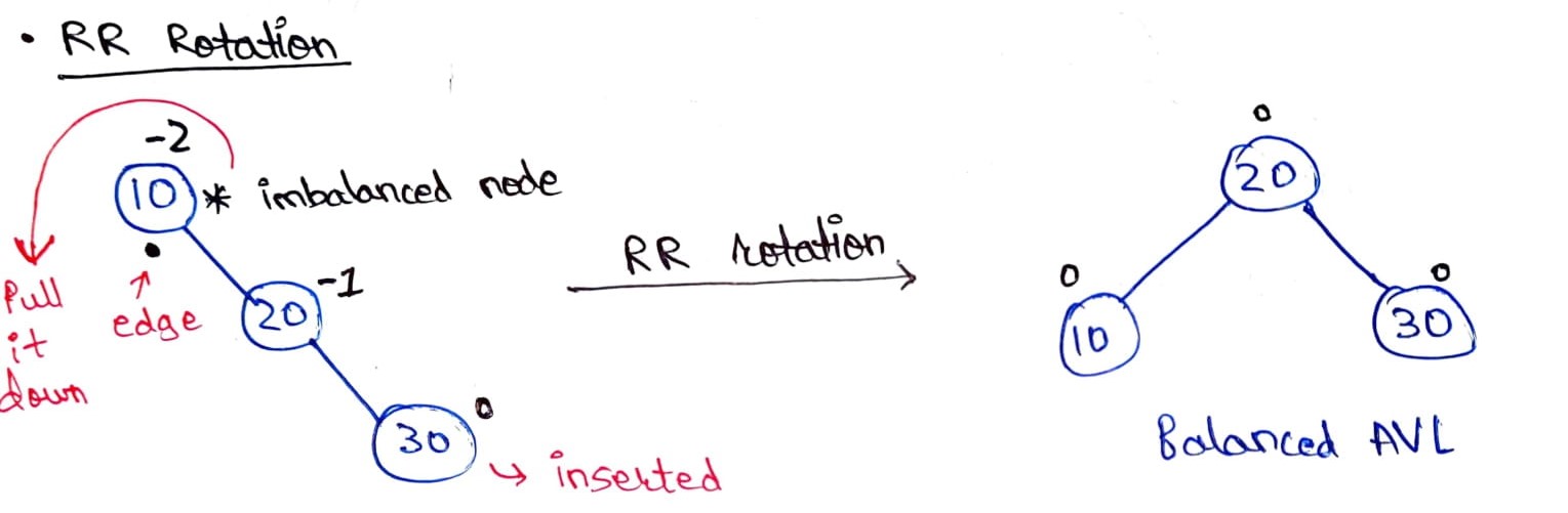
### 2. RR Rotation

It is similar to that of LL Rotation but in this case, the tree gets unbalanced, upon insertion of a node into the right subtree of the right child of the imbalance node i.e., upon **Right-Right (RR)** insertion instead of the LL insertion. In this case, the tree becomes right heavy and a **left rotation (or anti-clockwise rotation)** is performed along the edge of the imbalanced node to counter this right skewness caused by the insertion operation. Let’s understand this process with an example:

Consider a case where we wish to create a BST using the elements 10, 20, and 30. Now, since the elements are given in sorted order, the BST so created becomes right-skewed as shown below:

:::section{.graphics}
:::

Upon calculating the balance factor of all the nodes, we can confirm that the root node of the tree is imbalanced `(balance factor = 2)` when the element `30` is inserted using RR-insertion. Hence, the tree is heavier on the right side and we can balance it by transferring the imbalanced node on the left side by applying an anti-clockwise rotation around the edge (pivot point) of the imbalanced node or in this case, the root node.
:::

:::section{.sub-section}
### 3. LR Rotation

So far we have discussed that when the tree is heavy on one side, just perform a single rotation in the opposite direction to counter the effect of tree skewness. But, there also exist some cases where a single tree rotation isn’t enough to balance the tree i.e., we may need to perform one more rotation to finally counter the effects of the height-affecting operation.

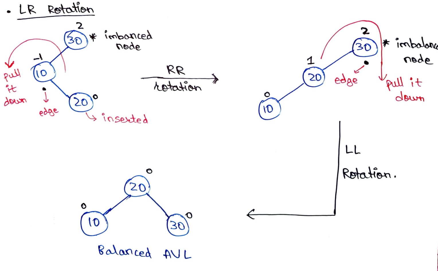
One such case is of **Left-Right (LR) insertion** i.e., the tree gets unbalanced, upon insertion of a node into the right subtree of the left child of the imbalance node. Let’s understand this case using an example:

Consider a situation where you create a BST using elements 30, 10, and 20. Now, when the elements are inserted, the element `30` becomes the root, `10` becomes its left child, and when the element `20 `is inserted, it is inserted as the right child of the node having the value `10`. This causes an imbalance in the tree as the root node’s balance factor becomes equal to `2`.

Now, as per the previous discussions, you may have noticed that a positive balance factor indicates that the given node is **left-heavy** while a negative one indicates that the node is **right-heavy**. Now, if we notice the immediate parent of the inserted node, we notice that its balance factor is negative i.e., its right-heavy. Hence, you may say that we should perform a left rotation (RR rotation) on the immediate parent of the inserted node to counter this effect. Let’s perform this rotation and notice the change:

:::section{.graphics}
:::

As you can observe, upon applying the RR rotation the BST becomes left-skewed and is still unbalanced. This is now the case of LL rotation and by rotating the tree along the edge of the imbalanced node in the clockwise direction, we can retrieve a balanced BST.

Hence, a simple rotation won’t fully balance the tree but it may flip the tree in such a manner that it gets converted into a single rotation scenario, after which we can balance the tree by performing one more tree rotation. This process of applying two rotations sequentially one after another is known as **double rotation** and since in our example the insertion was **Left-Right (LR) insertion**, this combination of RR and LL rotation is known as LR rotation. Hence, to summarize:

The LR rotation consists of two steps:
1. Apply RR Rotation (anti-clockwise rotation) on the left subtree of the imbalanced node as the left child of the imbalanced node is right-heavy. This process flips the tree and converts it into a left-skewed tree.
2. Perform LL Rotation (clock-wise rotation) on the imbalanced node to balance the left-skewed tree.

Hence, LR rotation is essentially a combination of RR and LL Rotation.
:::

:::section{.sub-section}
### 4. RL Rotation

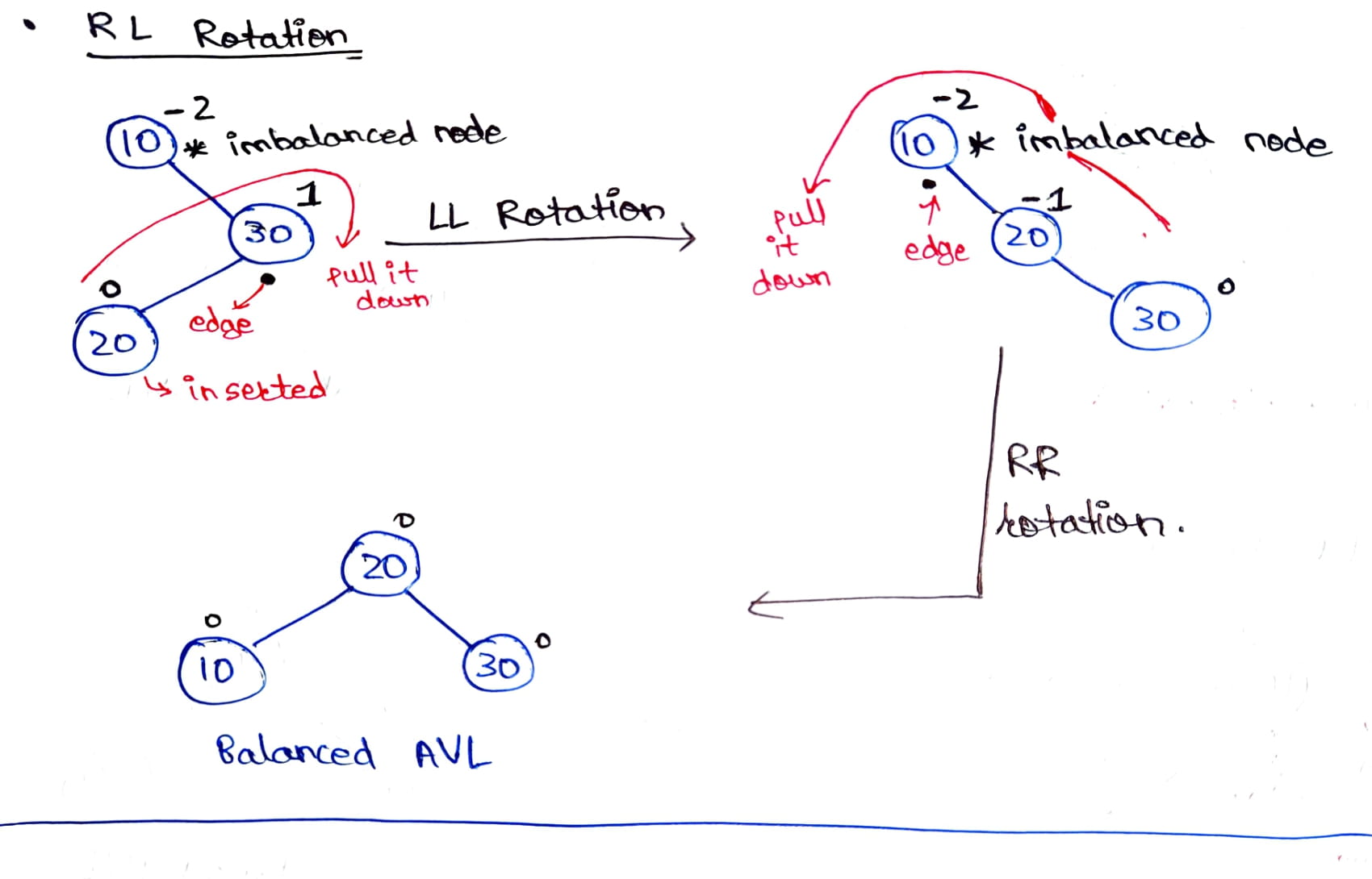
It is similar to LR rotation but it is performed when the tree gets unbalanced, upon insertion of a node into the left subtree of the right child of the imbalance node i.e., upon **Right-Left (RL) insertion** instead of LR insertion. In this case, the immediate parent of the inserted node becomes left-heavy i.e., the LL rotation (right rotation or clockwise rotation) is performed that converts the tree into a right-skewed tree. After which, RR rotation (left rotation or anti-clockwise rotation) is applied around the edge of the imbalanced node to convert this right-skewed tree into a balanced BST.

Let’s now observe an example of the RL rotation:

:::section{.graphics}
:::

In the above example, we can observe that the root node of the tree becomes imbalanced upon insertion of the node having the value `20`. Since this is a type of RL insertion, we will perform LL rotation on the immediate parent of the inserted node thereby retrieving a right-skewed tree. Finally, we will perform RR Rotation around the edge of the imbalanced node (in this case the root node) to get the balanced AVL tree.

Hence, RL rotation consists of two steps:
1. Apply LL Rotation (clockwise rotation) on the right subtree of the imbalanced node as the right child of the imbalanced node is left-heavy. This process flips the tree and converts it into a right-skewed tree.
2. Perform RR Rotation (anti-clockwise rotation) on the imbalanced node to balance the right-skewed tree.

:::

:::section{.tip}
**NOTE -**
- Rotations are done only on three nodes (including the imbalanced node) irrespective of the size of the Binary Search Tree. Hence, in the case of a large tree always focus on the two nodes around the imbalanced node and perform the tree rotations.
- Upon insertion of a new node, if multiple nodes get imbalanced then traverse the ancestors of the inserted node in the tree and perform rotations on the first occurred imbalanced node. Continue this process until the whole tree is balanced. This process is knowns as **retracing** which is discussed later in the article.

:::

:::section{.highlights}
**Highlights:**
1. Rotations are performed to maintain the AVL Balance criteria.
1. Rotation is a process of changing the structure without affecting the elements' order.
1. Rotations are done on an unbalanced node based on the location of the newly inserted node.
1. Single rotations include LL (clockwise) and RR (anti-clockwise) rotations.
1. Double rotations include LR (RR + LL) and RL (LL + RR) rotations.
1. Rotations are done only on 3 nodes, including the unbalanced node.

:::
::::::

::::::section{.main}
## Operations on AVL Trees

Since AVL Trees are self-balancing Binary Search Trees, all the operations carried out using AVL Trees are similar to that of Binary Search Trees. Also, since searching an element and traversing the tree doesn't lead to any change in the structure of the tree, these operations can't violate the height balancing property of AVL Trees. Hence, searching and traversing operations are the same as that of Binary Search Trees.

However, upon the execution of each insertion or deletion operation, we perform a check on the balance factor of all the nodes and perform rotations to balance the AVL Tree if needed. Let's look at these operations in detail:

:::section{.sub-section}
### 1. Insertion

In Binary Search Trees, the new node (let say `N`) was inserted in the tree by traversing the tree using BST logic i.e., comparing the value of `N` with the value of a node at each level and determining whether to traverse the right subtree (if `N` is greater) or the left subtree (if `N` is smaller) of the current traversed node. This traversal is done to locate a node having `NULL` as its child that can be replaced to insert the new node `N`. Hence, in BSTs a new node is always inserted as a leaf node by replacing the` NULL` value of a node’s child.

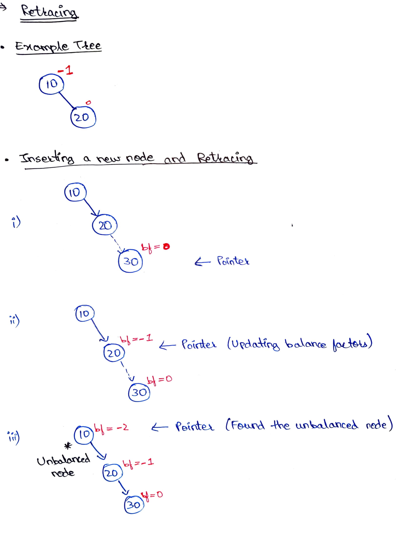
Just like the insertion in BSTs, the new node is always inserted as a leaf node in AVL Trees i.e., the balance factor of the newly inserted node is always equal to `0`. However, after each insertion in the tree, the balance factor for the ancestors of the newly inserted node is checked to verify that the tree is balanced or not. Here, only the ancestors of the inserted node are checked for imbalance because when a new node is inserted, it only alters the height of its ancestors thereby inducing an imbalance in the tree. This process of finding the unbalanced node by traversing the ancestors of the newly inserted node is known as **retracing**. If the tree becomes unbalanced after inserting a new node, retracing helps us in finding the location of a node in the tree at which we need to perform the tree rotations to balance the tree.

The below gif demonstrates the retracing process upon inserting a new element in the AVL Tree:

:::section{.graphics}
:::

Let’s look at the algorithm of the insertion operation in AVL Trees:

:::section{.tip}
**Insertion in AVL Trees**
1. START
1. Insert the node using BST insertion logic.
1. Calculate and check the balance factor of each node.
1. If the balance factor follows the AVL criterion, go to step 6
1. Else, perform tree rotations according to the insertion done. Once the tree is balanced go to step 6.
1. END

:::

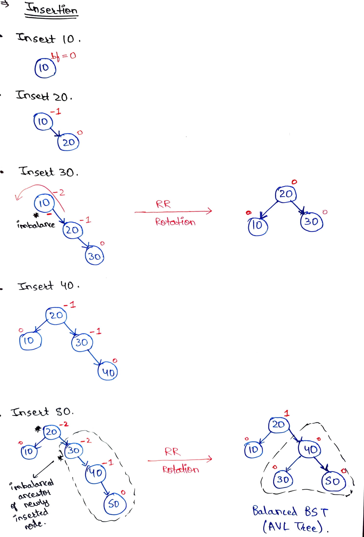
For better understanding let’s consider an example where we wish to create an AVL Tree by inserting the elements: 10, 20, 30, 40, and 50. The below gif demonstrates how the given elements are inserted one by one in the AVL Tree:

:::section{.graphics}
:::

:::

:::section{.sub-section}
### 2. Deletion

When an element is to be deleted from a Binary Search Tree, the tree is searched using various comparisons via the BST rule i.e., the left subtree is checked if the specified element is smaller than that of the current node, otherwise, the right subtree is checked till the current node has the same value as that of the specified element. If the element is found in the tree, there are three different cases in which the deletion operation occurs depending upon whether the node to be deleted has any children or not:

**Case 1: When the node to be deleted is a leaf node**
- In this case, the node to be deleted contains no subtrees i.e., it’s a leaf node. Hence, it can be directly removed from the tree.

**Case 2: When the node to be deleted has one subtree**
- In this case, the node to be deleted is replaced by its only child thereby removing the specified node from the BST.

**Case 3: When the node to be deleted has both the subtrees.**
- In this case, the node to be deleted can be replaced by one of the two available nodes:
- It can be replaced by the node having the largest value in the left subtree **(Longest left node or Predecessor)**.
- Or, it can be replaced by the node having the smallest value in the right subtree **(Smallest right node or Successor)**.

Just like the deletion operation in Binary Search Trees, the elements are deleted from AVL Trees depending upon whether the node has any children or not. However, upon every deletion in AVL Trees, the balance factor is checked to verify that the tree is balanced or not. If the tree becomes unbalanced after deletion, certain rotations are performed to balance the Tree.

Let’s look at the algorithm of the deletion operation in AVL Trees:

:::section{.tip}
**Deletion in AVL Trees**
1. START
1. Find the node in the tree. If the element is not found, go to step 7.
1. Delete the node using BST deletion logic.
1. Calculate and check the balance factor of each node.
1. If the balance factor follows the AVL criterion, go to step 7.
1. Else, perform tree rotations to balance the unbalanced nodes. Once the tree is balanced go to step 7.
1. END

:::

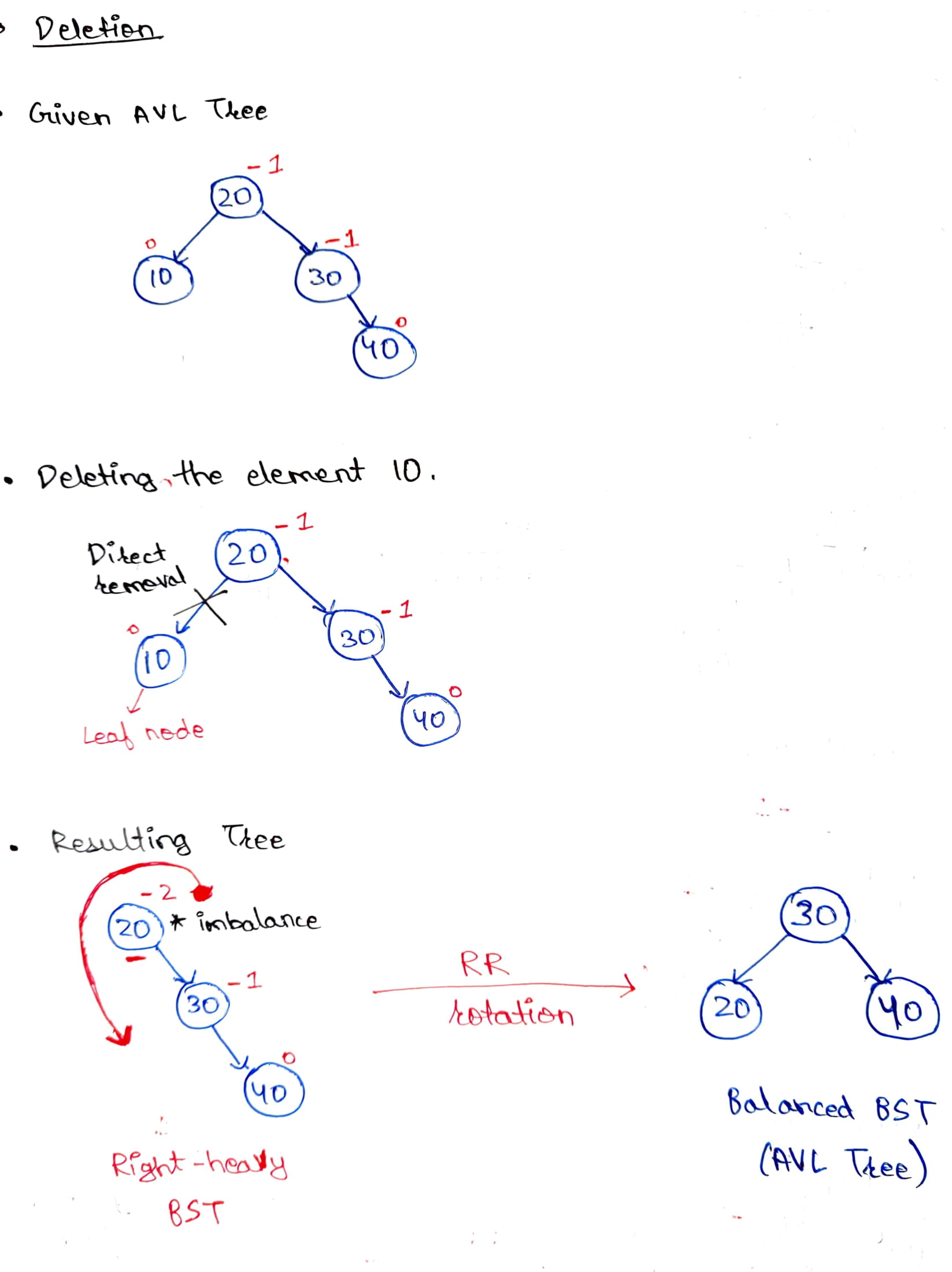
For better understanding let’s consider an example where we wish to delete the element having value `10` from the AVL Tree created using the elements 10, 20, 30, and 40. The below gif demonstrates how we can delete an element from an AVL Tree:

:::section{.graphics}
:::

:::

:::section{.highlights}
**Highlights:**
1. All AVL Tree operations are similar to that of BST except insertion and deletion.
1. Upon every insertion and deletion, we need to check whether the tree is balanced or not.
1. If required, the rotations are performed after each operation to balance the tree.

:::
::::::

::::::section{.main}
## Implementation

As we know that a tree is a recursive data structure as they are usually composed of smaller trees (subtrees) inside of them. Hence, we can make the implementation of a tree more effective by making use of the recursion process. The AVL tree data structure can be implemented using different methods such as using arrays or by using the object-oriented programming (OOPS) concept. Out of these two methods, the most suitable way to represent and implement a tree is by using the OOPS concept because when a tree is implemented using arrays the benefits of dynamic memory allocation are lost.

Hence, to implement AVL Trees we will create two classes (templates of objects) i.e., the Node class and the AVL class where the node class represents the node of the tree while the AVL class describes the behavior of the AVL tree that contains various Node objects. The AVL Tree node can be represented as:

Class Node {
    int data;
    int height;
    Node left_child;
    Node right_child;
};

Here, the Node class consists of the integer data variable that represents the value stored in the node, the height variable that is used to determine the height of the node, the left_child and right_child variables that are used to store the left and the right children of a given node.

Now, let’s consider an example in which we will create an AVL Tree using values: 10, 20, and 30. Since these elements are in sorted order, they all will be inserted in the right subtree of the previous element. Hence, the tree will become right-skewed and an RR rotation will be required to balance the tree. The resulting AVL Tree has 20 at its root and 10 and 30 as its left and right child respectively as shown below:

:::section{.graphics}
:::

Let’s understand how the above example is implemented using the OOPS concept:

- Firstly, we will create a class Node as described above to represent a node of the AVL Tree.
- Now, we will create another class AVL that represents the AVL Tree. This class will contain the following methods:
- **get_height(Node object):** This method will return the height of the Node object.
- **get_balance_factor(Node object):** This method is used to calculate the balance factor of the specified Node object.
- **pre_order(Node root):** This method is used to print the elements of the AVL tree using the pre-order traversal technique.
- **LL_rotation(Node object):** This method is used to perform LL rotation on the specified imbalanced node.
- **RR_rotation(Node object):** This method is used to perform RR rotation on the specified imbalanced node.
- **insert(Node object, int value):** It is a recursive function that is used to insert a node in the AVL tree.

Now, let's look at the implementation of the above discussed example in C++ and Java:

:::section{.sub-section}
### **AVL Tree in Java**

class Node {
    int data, height;
    Node left_child, right_child;

    Node(int val){
        data = val;
        height = 0;
    }
}

class avl {
    Node node;

    int get_height(Node root){
        if(root == null)
            return -1;
        return root.height;
    }

    int get_balance_factor(Node root){
        if(root == null)
            return 0;
        return (get_height(root.left_child) - get_height(root.right_child));
    }

    // Clockwise Rotation
    Node LL_rotation(Node root){
        Node child = root.left_child;
        root.left_child = child.right_child;
        child.right_child = root;
        root.height = Math.max(get_height(root.left_child), get_height(root.right_child)) + 1;
        child.height = Math.max(get_height(child.left_child), get_height(child.right_child)) + 1;
        return child;
    }

    // Anti-Clockwise Rotation
    Node RR_rotation(Node root){
        Node child = root.right_child;
        root.right_child = child.left_child;
        child.left_child = root;
        root.height = Math.max(get_height(root.left_child), get_height(root.right_child)) + 1;
        child.height = Math.max(get_height(child.left_child), get_height(child.right_child)) + 1;
        return child;
    }

    // Pre-order traversal of the tree
    void pre_order(Node root) {
        if (root != null) {
            System.out.print(root.data + " ");
            pre_order(root.left_child);
            pre_order(root.right_child);
        }
    }

    // AVL Insertion
    Node insert(Node root, int val){
        // BST Insertion Logic
        if (root == null)
            return (new Node(val));
        if (val < root.data)
            root.left_child = insert(root.left_child, val);
        else if (val > root.data)
            root.right_child = insert(root.right_child, val);
        else
            return node;

        // Balance Factor check
        root.height = Math.max(get_height(root.left_child), get_height(root.right_child)) + 1;
        int b = get_balance_factor(root);

        // Checking if the node insertion results in Left heavy or Right heavy nodes.
        if(b > 1){
            // LL Rotation Case
            if(get_balance_factor(root.left_child) == 1){
                root = LL_rotation(root);
            }
            // LR Rotation Case
            else{
                root.left_child = RR_rotation(root.left_child);
                root = LL_rotation(root);
            }
        }
        else if(b < -1){
            // RR Rotation Case
            if(get_balance_factor(root.right_child) == -1){
                root = RR_rotation(root);
            }
            // RL Rotation Case
            else{
                root.right_child = LL_rotation(root.right_child);
                root = RR_rotation(root);
            }
        }
        return root;
    }

    public static void main(String[] args) {
        avl tree = new avl();
        tree.node = tree.insert(tree.node, 10);
        tree.node = tree.insert(tree.node, 20);
        tree.node = tree.insert(tree.node, 30);
        System.out.println("Pre-order Traversal of the AVL Tree is : ");
        tree.pre_order(tree.node);
    }
}

:::

:::section{.sub-section}
### **AVL Tree in C++**

#include<bits/stdc++.h>
using namespace std;
class Node
{   public:
        int data, height;
        Node * left_child;
        Node * right_child;
};

class avl{
    public:
        Node * node = NULL;

        int get_height(Node * root){
            if(root == NULL)
                return -1;
            return (root->height);
        }

        int get_balance_factor(Node * root){
            if(root == NULL)
                return 0;
            return (get_height(root->left_child) - get_height(root->right_child));
        }

        // Clockwise Rotation
        Node * LL_rotation(Node * root){
            Node * child = root->left_child;
            root->left_child = child->right_child;
            child->right_child = root;
            root->height = max(get_height(root->left_child), get_height(root->right_child)) + 1;
            child->height = max(get_height(child->left_child), get_height(child->right_child)) + 1;
            return child;
        }

        // Anti-Clockwise Rotation
        Node * RR_rotation(Node * root){
            Node * child = root->right_child;
            root->right_child = child->left_child;
            child->left_child = root;
            root->height = max(get_height(root->left_child), get_height(root->right_child)) + 1;
            child->height = max(get_height(child->left_child), get_height(child->right_child)) + 1;
            return child;
        }

        // Pre-order traversal of the tree
        void pre_order(Node * root)
        {   if(root != NULL)
            {   cout << root->data << " ";
                pre_order(root->left_child);
                pre_order(root->right_child);
            }
        }

        // AVL Insertion
        Node * insert(Node * root, int new_data)
        {
            // BST Insertion Logic
            if(root == NULL){
                root = new Node;
                root->data = new_data;
                root->left_child = NULL;
                root->right_child = NULL;
                root->height = 0;
                return root;
            }
            if(root->data < new_data)
                root->right_child = insert(root->right_child, new_data);
            else
                root->left_child = insert(root->left_child, new_data);

            // Balance Factor Check
            root->height = max(get_height(root->left_child), get_height(root->right_child)) + 1;
            int b = get_balance_factor(root);

            // Checking if the node insertion results in Left heavy or Right heavy nodes.
            if(b > 1){
                // LL Rotation Case
                if(get_balance_factor(root->left_child) == 1){
                    root = LL_rotation(root);
                }
                // LR Rotation Case
                else{
                    root->left_child = RR_rotation(root->left_child);
                    root = LL_rotation(root);
                }
            }
            else if(b < -1){
                // RR Rotation Case
                if(get_balance_factor(root->right_child) == -1){
                    root = RR_rotation(root);
                }
                // RL Rotation Case
                else{
                    root->right_child = LL_rotation(root->right_child);
                    root = RR_rotation(root);
                }
            }
            return root;
        }
};

int main()
{   avl tree;
    tree.node = tree.insert(tree.node, 10);
    tree.node = tree.insert(tree.node, 20);
    tree.node = tree.insert(tree.node, 30);
    cout << "Pre-order Traversal of the AVL Tree is : ";
    tree.pre_order(tree.node);
    return 0;
}

:::

The output of all the above given implementations is same and is shown below:

**Output:**

Pre-order Traversal of the AVL Tree is : 20 10 30 

::::::

::::::section{.main}
## Complexity of AVL Tree

The complexity of a data structure is measured based on the time taken by certain operations performed using that data structure and the space required to efficiently execute those operations. Therefore, the complexity includes:

:::section{.sub-section}
### **Time Complexity**

Let’s take a look at the time complexity of different operations performed using the AVL Trees:

**Traversal**
Traversing is the process of accessing all the nodes present in the tree i.e., we need to visit all the nodes of the tree. Hence, for the n number of nodes present in the tree, the time complexity will always be `O(n)`.

**Searching**
Searching is the process of finding an element in the tree. As discussed earlier, the searching process doesn’t affect the height of the tree, Hence searching in AVL Tree is exactly the same as that in BST i.e., we always start searching from the root node and perform comparisons to find out the location of the element in the tree. But, since in AVL Trees the height is always balanced, we are reducing the comparison operations by half at each level as we traverse down the tree. Hence, the time complexity of searching operation using the AVL Trees is `O(log n)`, where `n` is the number of nodes present in the tree.

**Insertion**
Insertion is the process of adding a new node in the tree. Since we perform three sub-operations one by one in insertion, we need to consider the time taken by these sub-operations to evaluate the overall time complexity. These sub-operations include:

- Finding the location of the insertion by performing BST logic-based comparisons at each level of the tree.
- Inserting the node and calculating the balance factor of retraced nodes.
- Performing tree rotations if required.

Now, out of the above-mentioned sub-operations, The rotation process takes constant time as only 3 nodes are affected by the rotation. Also, the balance factor calculation and the retracing process take constant time. Hence, the time complexity of insertion depends only upon the process of finding the location of insertion which depends on the height of the tree (discussed earlier in the article). Therefore, the time complexity for insertion in AVL Tree is `O (log n)` as the AVL Tree is height-balanced and attains minimal height i.e., `O (log n)`.

**Deletion**
Deletion is the process of removing a node from the tree. Similar to insertion, in the deletion process we also need to search the tree to locate the node to be deleted, then calculate the balance factor for retraced nodes, and perform rotations if required. Hence, deletion operation also depends on the searching time i.e., the time complexity for deletion from an AVL Tree is also `O (log n)`, where `n` is the total number of nodes present in the tree.

:::

:::section{.sub-section}
### **Space Complexity**

The AVL Trees can be considered as a Binary Search Tree having height-balancing property. This height-balancing property is achieved by changing the structure of the BST using tree rotations. Hence, in AVL Trees we are only changing the structure of the data and not the data itself. Hence, its space complexity is the same as that of Binary Search Trees i.e., `O (n)` as the BSTs can be visualized as a sorted linear array data structure having `n` number of elements.

:::

:::section{.highlights}
**Highlights:**
1. AVL Trees are always balanced i.e., their height remains `O(log n)`.
2. AVL Trees can balance themselves by only changing the structure of the tree.
3. Because of AVL Trees' balanced height, the time complexity of certain operations are:
| Operation | Average-Case | Worst-Case |
|:---------:|:------------:|:----------:|
| Traversal | O (n) | O(n) |
| Searching | O (log n) | O(log n) |
| Insertion | O (log n) | O(log n) |
| Deletion | O (log n) | O(log n) |
4. Space complexity is same as that of BSTs i.e., `O (n)` as AVL Trees doesn't modify the data itself.

:::
::::::

:::section{.main}
## Advantages of AVL Tree

AVL Trees were developed to overcome the dependency of operations on the height of the Binary Search Tree and the inability to control the tree's height. Hence, the main advantage of AVL Trees include:

- It can be used to perform searching operations on dynamic data sets, just like Binary Search Trees.
- Its height is always balanced i.e., it always stays as a balanced BST which has minimal or logarithmic or O (log n) height, where n is the total number of nodes present in the tree.
- It has a self-balancing property which is implemented by calculating the balance factor of all the nodes after each operation and performing certain Tree rotations to make sure that all the nodes follow the AVL Balancing criteria.
- Because of the self-balancing property, the AVL Tree remains height-balanced and it performs way better than BSTs by performing operations in logarithmic time complexity, especially when the number of nodes present in the tree is very large.
- Because of the logarithmic time complexity, the searches performed using AVL trees are faster and more reliable than that of BSTs.

:::section{.highlights}
**Highlights:**
1. Can be used to search dynamic datasets
1. Maintains its height by performing rotations whenever the balance factor of a node violates the Balancing Criteria. As a result, it has self-balancing properties.
1. Exists as a balanced BST at all times, providing logarithmic time complexity for operations such as searching.
1. Provides faster and reliable searching than BSTs, especially when the number of nodes present is very large.

:::
:::

:::section{.conclusion}
## Conclusion

- AVL Tree is a self-balancing Binary Search Trees.
- It exhibits self-balancing by associating each node with a balance factor.
- It is faster than BST and performs all operations in logarithmic time.
- Balance factor indicates whether a node is left heavy, right heavy, or balanced.
- For a balanced AVL tree, the absolute balance factor of all the nodes should not be greater than unity. (AVL Balance Criteria)
- To balance the tree, certain tree rotations are used based on the operations that caused the imbalance.
- Rotations are changes in the structure of the tree, done only on 3 nodes without affecting the elements' order.
- Single Rotations include LL (clockwise) and RR (anti-clockwise).
- Double rotations include LR (RR + LL) and RL (LL + RR) rotations.
- All AVL Tree operations are similar to BST except insertion and deletion.

:::