# Optimizing nested neighbor accesses in ICON
## Inlining in a cartesian context
Cartesian stencil computations are well understood and well optimized across different hardware platforms (CPU, GPU, FPGA, ...).
Under the correct circumstances, inlining proves to be excellent optimization for cartesian stencil computations (see [domain-specific-rewriting] of [gridtools]). For example, in the the following GT4Py code snippet, two `field_operator`s `laplace` and `centered_difference_i`
```python=
@gtx.field_operator
def laplace(
in_field: gtx.Field[[I, J], float]
) -> gtx.Field[[I, J], float]:
return (
-4.0 * in_field,
+ in_field(I + 1, J + 1),
+ in_field(I + 1, J - 1),
+ in_field(I - 1, J + 1),
+ in_field(I - 1, J - 1),
)
```
```python=
@gtx.field_operator
def centered_difference_i(
in_field: gtx.Field[[I, J], float]
) -> gtx.Field[[I, J], float]:
return in_field(I + 1) - in_field(I - 1)
```
can be combined by calling them in series, as in the following stencil:
```python=
@gtx.field_operator
def combined_serial(
in_field: gtx.Field[[I, J], float]
) -> gtx.Field[[I, J], float]:
tmp = laplace(in_field)
return centered_difference_i(tmp)
```
But they can also be inlined to prevent an intermediate result to be written to RAM, potentially resulting in a speedup since stencil computations for weather and climate simulations are usually memory bound.
```python=
@gtx.field_operator
def combined_naive(
in_field: gtx.Field[[I, J], float]
) -> gtx.Field[[I, J], float]:
return (
- 4.0 * in_field(I + 1)
+ in_field(I + 2, J + 1)
+ in_field(I + 2, J - 1)
+ in_field( J + 1)
+ in_field( J - 1)
+ 4.0 * in_field(I - 1)
- in_field( J + 1)
- in_field( J - 1)
- in_field(I - 2, J + 1)
- in_field(I - 2, J - 1)
)
```
### Inlining for the icosahedral mesh

The icosahedral mesh used in [ICON](https://www.icon-model.org/) (Icosahedral non-hydrostatic model) consists of 12 pentagons (5 triangles around a vertex) and as many hexagons (6 triangles around a vertex) as necessary to arrive at the desired resolution.

Illustration by Günther Zängl
In the computational model we have fields that exists on the cell, fields that exists on the edges and some fields that exists on the vertices.
For that reason neighbor accesses, for example for a 2nd order accurate laplace operator, are not direct accesses, as in the cartesian case, but they involve lookup tables for the correct address of your neighbor. For example, every edge in the mesh has 2 direct cell neighbors.
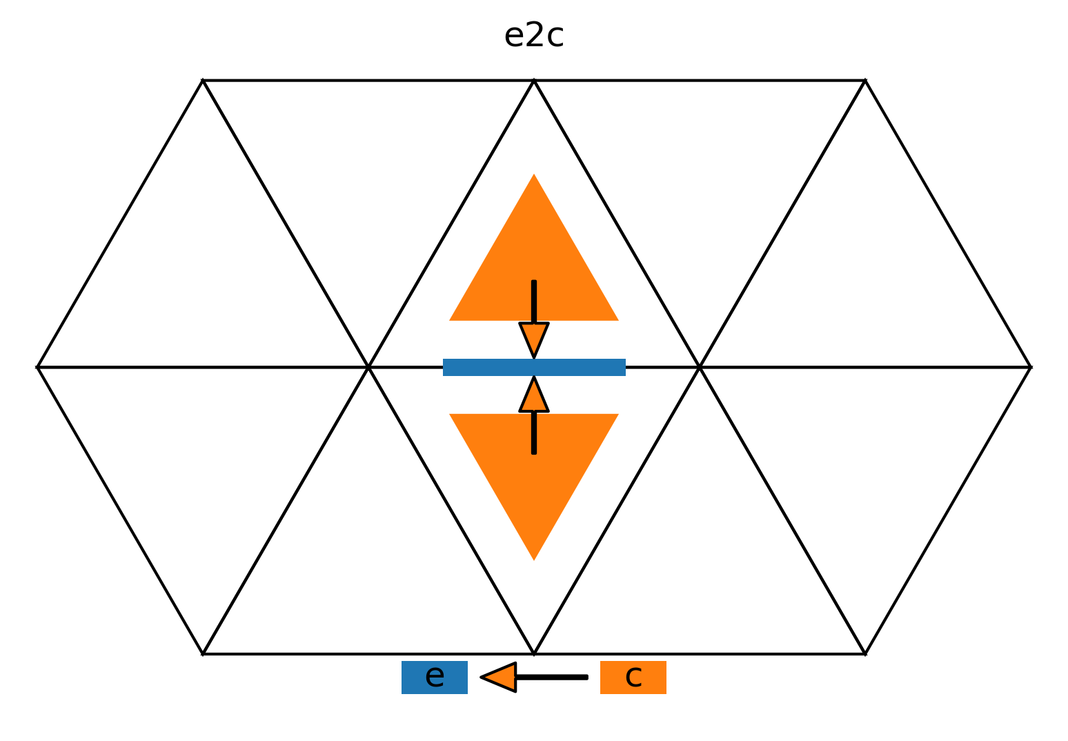
Illustration by Jacopo Canton
We call these neighbor access patterns neighbor reductions in case of a pattern where the weighted sum of all direct neighbors is computed.
If two or more of these neighbor access patterns directly follow each other, they can be combined into one operation, similarly to how we combined the `laplace` and the `centered_difference_i` above for the Cartesian case.
#### Inlining two neighbor accesses in consecutive stencils
Naively inlining a neighbor reduction into another will result in the same elements of a vector being accessed over different pointer tables, leading to unnecessary loads, as we can see in the following example.
The goal of the following computation is to compute a value on the edge in the center of the image, marked in blue. To compute the value on the edge, we want to sum over the values of the 4 vertices closest to the edge. We have no way of accessing these four vertices directly, so we have to go over the two neighbor cells of the edge and request a list of vertices from each of the two cells.
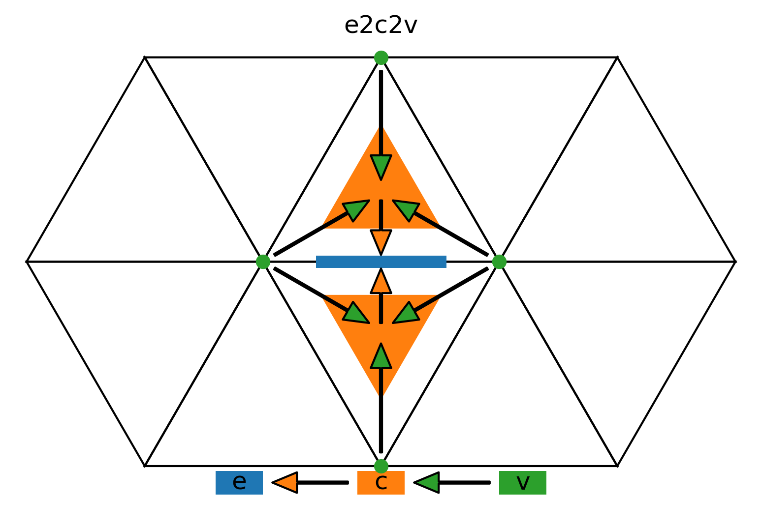
Illustration by Jacopo Canton
```python=
@field_operator
fn c2v_stencil(
vertex_input: VertexKField[float]
) -> CellKField[float]
return neighbor_sum(vertex_input(C2V), axis=C2VDim)
@field_operator
fn e2c_stencil(
cell_input: CellKField[float]
) -> EdgeKField[float]
return neighbor_sum(cell_input(E2C), axis=E2CDim)
@field_operator
fn e2c2v_stencil(
vertex_input: VertexKField[float]
) -> EdgeKField[float]
tmp = c2v_stencil(vertex_inmput)
return e2c_stencil(tmp)
```
The resulting list of 6 vertices (3 from each cell) is however redundant, two of the vertices are listed twice.
```c=
for(edge = 0; edge < num_edge, edge++)
{
vertex_input(c2v(0, e2c(0, edge)))
+
vertex_input(c2v(1, e2c(0, edge)))
+
vertex_input(c2v(2, e2c(0, edge)))
+
vertex_input(c2v(0, e2c(1, edge)))
+
vertex_input(c2v(1, e2c(1, edge)))
+
vertex_input(c2v(2, e2c(1, edge)))
}
```
However, with our naive code we have no way of knowing which of the vertices are duplicates of each other.
With domain specific knowledge about the ICON mesh we can deduplicate the memory accesses in the following way:
```c=
vertex_input(c2v(1, e2c(0, edge))) == vertex_input(c2v(0, e2c(1, edge)))
vertex_input(c2v(2, e2c(0, edge))) == vertex_input(c2v(1, e2c(1, edge)))
```
```c=
for(edge = 0; edge < num_edge, edge++)
{
vertex_input(e2v(0, edge))
+
vertex_input(e2v(1, edge))
+
vertex_input(e2v(2, edge))
+
vertex_input(e2v(1, edge))
+
vertex_input(e2v(2, edge))
+
vertex_input(e2v(3, edge))
}
```
### Task:
On an idealized hexagonal mesh:
* Automate the nested neighbor reduction in the gt4py and/or DaCe compiler(s) for all relevant combinations of dimensions (`Edge`, `Cell` and `Vertex`) for neighbor chain lenghts of 3 (possibly 4) (example length 3:`Edge` to `Cell` to `Vertex`, can be written as `E2C2V`)
* Do a performance analysis on the resulting code, come up with an algorithm/heuristic to estimate when the optimization is worth doing and when not, probably using the number of data loads of the inilined and serial execution as predictor (this algorithm/heuristic does not need to take into account all relevant information, such as what kind of space filling curve is used in the mesh.)
* Generalize the nested neighbor reduction pass to be able to look across multiple kernels in order to find opportunities to apply the optimization
* (Stretch goal) Come up with a set of constraints for the neighborhood tables so that generating direct access tables for neighborhood chains is always consistent for hexagonal mesh or show that it is impossible.
On the icosahedral ICON grid (icon-nwp or EXCLAIM):
* (Stretch goal) Evaluate the performance of the optimizations
* (Stretch goal) Change the generated space filling curve, neighbor table order, ... in order to speed up the resulting code
* (Stretch goal) Come up with a set of constraints for the neighborhood tables so that generating direct access tables for neighborhood chains is always consistent for icosahedral mesh or show that it is impossible.
### Attachment: some more examples
#### Inlining two neighbor accesses in consecutive stencils (with sparse fields)
```python=
@field_operator
fn c2v_stencil(
vertex_input: VertexKField[float]
c2v_sparse: Field[[CellDim, C2VDim], float]
) -> CellKField[float]
return neighbor_sum(c2v_sparse * vertex_input(C2V), axis=C2VDim)
@field_operator
fn e2c_stencil(
cell_input: CellKField[float]
e2c_sparse: Field[[EdgeDim, E2CDim], float]
) -> EdgeKField[float]
return neighbor_sum(e2c_sparse * cell_input(E2C), axis=E2CDim)
@field_operator
fn e2c2v_stencil(
vertex_input: VertexKField[float]
c2v_sparse: Field[[CellDim, C2VDim], float]
e2c_sparse: Field[[EdgeDim, E2CDim], float]
) -> EdgeKField[float]
tmp = c2v_stencil(vertex_inmput, c2v_sparse)
return e2c_stencil(tmp, e2c_sparse)
```
```c=
for(edge = 0; edge < num_edge, edge++)
{
e2c_sparse(0, edge) *
c2v_sparse(0, e2c(0, edge)) *
vertex_input(c2v(0, e2c(0, edge)))
+
e2c_sparse(0, edge) *
c2v_sparse(1, e2c(0, edge)) *
vertex_input(c2v(1, e2c(0, edge)))
+
e2c_sparse(0, edge) *
c2v_sparse(2, e2c(0, edge)) *
vertex_input(c2v(2, e2c(0, edge)))
+
e2c_sparse(1, edge) *
c2v_sparse(0, e2c(1, edge)) *
vertex_input(c2v(0, e2c(1, edge)))
+
e2c_sparse(1, edge) *
c2v_sparse(1, e2c(1, edge)) *
vertex_input(c2v(1, e2c(1, edge)))
+
e2c_sparse(1, edge) *
c2v_sparse(2, e2c(1, edge)) *
vertex_input(c2v(2, e2c(1, edge)))
}
```
#### C2E + E2C = C2C with orientation
```python=
@field_operator
fn e2c_stencil(
cell_input: CellKField[float]
) -> EdgeKField[float]
return cell_input(E2C[1]) - cell_input(E2C[0])
@field_operator
fn c2e_stencil(
edge_input: EdgeKField[float]
) -> CellKField[float]
return neighbor_sum(edge_input(C2E), axis=C2EDim)
@field_operator
fn c2e2c_stencil(
cell_input: CellKField[float]
) -> CellKField[float]
tmp = e2c_stencil(cell_input)
return c2e_stencil(tmp)
```
```c=
for(cell = 0; cell < num_cell, cell++)
{
cell_field(e2c(0,(c2e(1, cell)))) - cell_field(e2c(0,(c2e(0, cell))))
+
cell_field(e2c(1,(c2e(1, cell)))) - cell_field(e2c(1,(c2e(0, cell))))
+
cell_field(e2c(2,(c2e(1, cell)))) - cell_field(e2c(2,(c2e(0, cell))))
}
```
This code cannot be substituted by the same code for every cell as long as the edge orientation in ICON is inconsistent.

[domain-specific-rewriting]: https://arxiv.org/abs/2005.13014 "Domain-Specific Multi-Level IR Rewriting for GPU"
[gridtools]: https://www.sciencedirect.com/science/article/pii/S2352711021000522 "GridTools: A framework for portable weather and climate applications"
 Sign in with Wallet
Connect another wallet
Sign in with Wallet
Connect another wallet