# Feature Engineering Note
- https://blog.csdn.net/v_JULY_v/article/details/81319999
## Feature Selection
- https://towardsdatascience.com/a-creative-approach-towards-feature-selection-b333dd46fe92
### Introduction
- Feature Selection is one of the most important things when it comes to feature engineering.
- We need to reduce the number of features so that we interpret the model better, make it less computational stressful to train the model, remove redundant effects and make the model generalise better.
- In some case feature selection becomes extremely important or else the input dimensional space is too big making it difficult for the model to train.
### Various ways to perform feature selection
1. Chi-Squared Test (categorical v.s. continuous variable)
2. Correlation Matrix (continuous v.s. continuous variable)
3. Domain knowledge
4. Coefficient of linear regularised models
5. Tree methods's feature importance (prefer this one the most)
### A Creative Approach Towards Feature Selection
- https://towardsdatascience.com/a-creative-approach-towards-feature-selection-b333dd46fe92
- Here the author propose a creative take on how to perform feature selection using all methods instead of being hinged into just one.
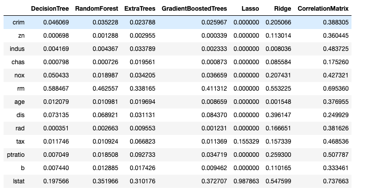
- The core idea is to combine correlation matrix (each variable is compared with the target variable), coefficient of linear regularised models and featur eimportance of various tree methods, combine them using randomly weighted average.
- Random weighting is used so that there is not inherent bias towards one kind of single approach.
- In the end, we have a final feature importance matrix having a mix of each of features selection approach on the go.
- It is always a nice thing to have a single output figure in front of us as compared to looking into various approaches.
#### Proof of Concept
To display the proof of concept I will use the Boston Housing Dataset. It is a regression case and all the input variable are continuous.
1. Firstly compute the correlation matrix for the whole dataset. Here only this is done because all the variable are continuous.
- In the case where there are some categorical variable we need to use **chi-square statistic** instead of correation matrix.
```python
correlation=abs(data.corr()['medv'])
del correlation['medv']
correlation.sort_values(ascending=True).plot(kind='barh')
plt.show()
```
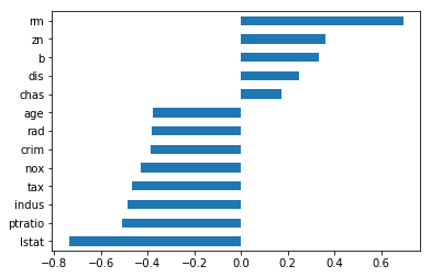
Natural values of linear correlation with respect to target variable
Absolute Linear correlation with respect to the target variable ‘MEDV’
2. Select Lasso and Ridge for computing coefficient of variable.
```python
from sklearn.preprocessing import MinMaxScaler
minmax=MinMaxScaler()
xScaled=minmax.fit_transform(X)
```
```python
lasso=Lasso()
lasso.fit(xScaled,Y)
lassocoeff = pd.Series((lasso.coef_), index=X.columns)
lassocoeff.sort_values(ascending=True).plot(kind='barh')
plt.show()
normLasso = lassocoeff/np.linalg.norm(lassocoeff)
normLasso = pd.Series(abs(normLasso), index=X.columns)
normLasso.sort_values(ascending=True).plot(kind='barh')
plt.show()
```
```python
ridge=Ridge()
ridge.fit(xScaled,Y)
ridgecoeff = pd.Series((ridge.coef_), index=X.columns)
ridgecoeff.sort_values(ascending=True).plot(kind='barh')
plt.show()
normRidge = RidgeCoeff/np.linalg.norm(RidgeCoeff)
normRidge = pd.Series(abs(normRidge), index=X.columns)
normRidge.sort_values(ascending=True).plot(kind='barh')
plt.show()
```
Lasso natural coefficients
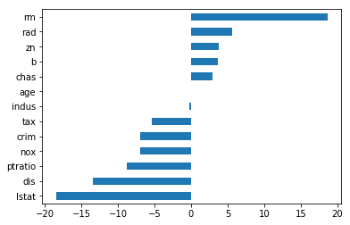
Ridge natural coefficients

Normalised and absolute values of lasso coefficients
Normalised and absolute values of ridge coefficients
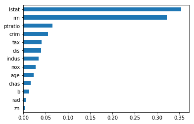
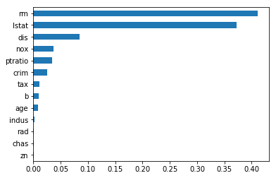
3. Select `GradientBoostingRegressor`, `RandomForestRegressor`, `DesitionTreeRegressor` and `ExtrTreeRegressor` for computing feature importance.
- In practice before this step all transformations of categorical variabls should be done (for instance either using one hot encoding or label encoding).
```python
dt=DecisionTreeRegressor()
dt.fit(X,Y)
feat_importances1 = pd.Series(dt.feature_importances_, index=X.columns)
feat_importances1.sort_values(ascending=True).plot(kind='barh')
plt.show()
```
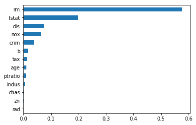
Decision Tree Feature Importance
```python
rf=RandomForestRegressor()
rf.fit(X,Y)
feat_importances2 = pd.Series(rf.feature_importances_, index=X.columns)
feat_importances2.sort_values(ascending=True).plot(kind='barh')
plt.show()
```

Random Forest Feature Importance
```python
et=ExtraTreesRegressor()
et.fit(X,Y)
feat_importances3 = pd.Series(et.feature_importances_, index=X.columns)
feat_importances3.sort_values(ascending=True).plot(kind='barh')
plt.show()
```
Extra Trees Feature Importance
```python
gbr=GradientBoostingRegressor()
gbr.fit(X,Y)
feat_importances4 = pd.Series(gbr.feature_importances_, index=X.columns)
feat_importances4.sort_values(ascending=True).plot(kind='barh')
plt.show()
```
Gradient Boosted Trees Feature Importance
```python
combinedDf = {
'DecisionTree': feat_importances1,
'RandomForest': feat_importances2,
'ExtraTrees': feat_importances3,
'GradientBoostedTrees': feat_importances4,
'Lasso':normLasso,
'Ridge':normRidge,
'CorrelationMatrix':abs(corr)}
```
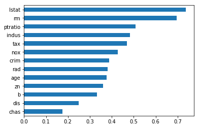
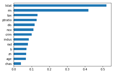
4. Use `numpy` for random sampling to give weights to each approach then take the weighted average.
```python
weight1= np.random.randint(1,10)/10
weight2= np.random.randint(1,10)/10
weight3= np.random.randint(1,10)/10
weight4= np.random.randint(1,10)/10
weight5= np.random.randint(1,10)/10
weight6= np.random.randint(1,10)/10
weight7= np.random.randint(1,10)/10
weightSum=weight1+weight2+weight3+weight4+weight5+weight6+weight7
```
```python
feat=(weight1*feat_importances1+weight2*feat_importances2+weight3*feat_importances3+weight4*feat_importances4+weight5*normLasso+weight6*normRidge+weight7*abs(corr))/(weightSum)
```
Here we have used a random weigth generation scheme where we don't 0 for any form of feature selection mechanism and the value of weights are in steps of 0.1 for simplecity.
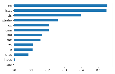
5. Then we return combined result which can be visualised using bar plot.
```python
feat.sort_values(ascending=True).plot(kind='barh')
plt.show()
```
### The 5 Feature Selection Algorithms every Data Scientist should know
- https://towardsdatascience.com/the-5-feature-selection-algorithms-every-data-scientist-need-to-know-3a6b566efd2
- Filter based
- Wrapper-based
- Embedded
- Pearson Correlation
- Chi-Squared
- Recursive Feature Elimination
- Lasso: SelectFromModel
- Tree-based: SelectFromModel
- RandomForest, XGBoost, LightGBM
- Bonus
## Dimension Reduction
### PCA
#### tutorial
- An overview of Principal Component Analysis
### t-SNE
https://towardsdatascience.com/why-you-are-using-t-sne-wrong-502412aab0c0
#### Overview
- While t-SNE is a dimensionality reduction technique, it is most used for **visualization** and not **data pre-processing** (like you might with PCA).
- For this reason, you almost always reduce the dimensionality down to 2 with t-SNE, so that you can then plot the data in two dimensions.
- The reason t-SNE is common for visualization is that the goal of the algorithm is to take your high dimensional data and represent it correctly in lower dimensions -- thus points that are close in high dimensions should remain close in low dimensions.
- It does this in a **non-linear and local way**, so different regions of data could be transformed differently.
- There is an incredibly good [article on t-SNE](https://distill.pub/2016/misread-tsne/) that discuess much of the above as well as the following points that you need to be award of:
1. **You cannot see the relative sizes of clusters in a t-SNE plot**. This point is crucial to understand as t-SNE naturally expands dense clusters and shrinks sparse ones.
2. ***Distance between well-separated clusters in a t-SNE plot may mean nothing***.
3. **Clumps of points -- especially with small perplexity values -- might just be noise**. It is vital to be careful when using small perplexity values for this reasion.
#### Characteristics
t-SNE has a hyper-parameter called **perplexity**. It balances the attention t-SNE gives to local and global aspects of the data and can have large effects on the resulting plot. A few notes on this parameter:
* It is roughly a guess of the number of close neighbors each point has. Thus, a denser dataset usually requires a higher perplexity value.
* It is recommended to be between 5 and 50.
* It should be smaller than the number of data points.
**The biggest mistake people make with t-SNE is only using one value for perplexity and not testing how the results change with other values**.
* If choosing different values between 5 and 50 significantly change your interpretation of the data, then you should consider other ways to visualize or validate your hypothesis.
It is also overlooked that since t-SNE uses gradient descent, you also have to tunr apropriate values for your learning rate and the number of steps for the optimizer. The key is to make sure the algorithm runs long enough to stabilize.
### UMAP
### CompressionVAE (CVAE)
https://towardsdatascience.com/compressionvae-a-powerful-and-versatile-alternative-to-t-sne-and-umap-5c50898b8696
#### Characteristics
- faster than either t-SNE or UMAP
- tends to learn a very smooth embedding space
- The learned representations are highly suitable as intermediate representations for downstream tasks
- CVAE learns a deterministic and reversible mapping from data to embedding space
- (note: the most recent version of UMAP also offers some reversibility)
- The tool can be integrated into live systems that can process previously unseen examples without re-training
- The trained systems are full generative models, and can be used to generate new data from arbitrary latent variables
- CVAE scales well to high dimensional input and latent spaces
- It can in principle scale to arbitrarily large datasets.
- highly customisable, even in its current implementation, giving many controllable parameters
- Beyond the current implementation, it is highly extensible, and future versions could provide for example convolutional or recurrent encoders/decoders to allow for more problem/data specific high quality embeddings beyond simple vectors.
- VAEs have a very strong and well studied theoretical foundation
- Due to the optimisation objective, CVAE often does not get a very strong separation between clusters.
##### Downside
- Biggest downside: As almost any deep learning tool, it needs a lot of data to be trained.
## Feature Scaling
- https://medium.com/towards-artificial-intelligence/feature-scaling-with-pythons-scikit-learn-10ab42119ae0
- There are four types of feature scaling in ```scikit-learn```:
- ```StandardScaler```
- It assumes your data is **normally distributed** within each feature and will scale scale them such that the distribution is now centered around 0, with and standard deviation of 1.
- The mean and standard deviation are calculated for the feature and then the feature is scaled base on:
$$
(x_i - mean(x)) / stdev(x)
$$
- If data is **not** normally distributed, this is not the best
- All feature are now on the same scale relative to on another:

- ```MinMaxScaler```
- Probably the most famous scaling algorithm, and follows the following formula for each feature:
$$
(x_i - min(x)) / (max(x) - min(x))
$$
- It essentially shrinks the range such that the range is now between 0 and 1 (or - 1 to 1 if there are negative values).
- Works better for cases in which the standard scaler might not work so well.
- If the distribution is not Gaussian or the standard deviation is very small, the min-max scaler works better.
- **Sensitive to outliers**
- You might want to use the ```Robust Scaler``` instead.
- Notice that the skewneww of the distribution is maintained but the 3 distrobutions are brought into the same scale so that they overlap:

- ```RobustScaler```
- Uses a similar method to the min-max scaler but it instead uses the interquartile range.
- It thus is robust to outliers.
- It follows the formula:
$$
(x_i - Q_i(x)) / (Q_3(x) - Q_1(x))
$$
for each feature.
- It is more suitable for when there are outliers in the data because it uses less of the data for scaling.
- Notice that after Robust scaling, the distributions are brought into the same scale and overlap:

- But the outliers remain outside of the bulk of the new distributions.
- However in min-max scaling, the two normal distributions are kept seperate by the outliers that are inside the 0-1 range.
- ```Normalizer```
- Scales each value by dividing each value by its magnitude in $N$-dimentional space for $N$ number of features.
- Say your features are x, y, and z Cartesian coordinates your scaled value for x would be:
$$
x_i/\sqrt{(x_{i}^{2} + y_{i}^{2} + z_{i}^{2})}
$$
- Each point is now within 1 unit of the origin on this Cartesian coordinate system.
- Note that the points are all brought within a sphere that is at most 1 away from the origin at any point. Also, the axes that are previously different scales are now all one scale:

## Manifold Learning
- https://towardsdatascience.com/step-by-step-signal-processing-with-machine-learning-manifold-learning-8e1bb192461c
- https://github.com/kayoyin/signal-processing
- A **manifold** is any space that is locally Euclidean.
- To put it simply, you can think of it as any object that is nearly "flat" on a small scale.
- Manifold leanring performs dimensionality reduction by representing data as a **low-dimensional** manifolds embedded in a higher-dimentional space.
### Isomap
- based on spectral theory to preserve geodesic distances
- distance of the **shortest path** between data points
- It can be understood as an extension of multi-dimensional scaling (MDS).
- First, compute the **distance matrix** of the dataset, obtain the **shortest paths** matrix and apply **MDS** on it.
- Next, like PCA, compute the **eigenvectors** and the corresponding **eigenvalues** of the centered distance matrix.
### Local Linear Enbedding (LLE)
- Idea: compute a **set of weights** to describe each data point as a **linear combination of its neighbors**.
- Then, it uses an eigenvector-based optimization technique to find the low-dimensional embedding such that the relations of linear combinations between points and its neighbors are **preserved**.
- Begin LLE by computing the distance matrix except we are interested in the points that are the **nearest neighbors** of each data point.
- Next, LLE finds the weight matrix *W* that minimizes the following cost function:
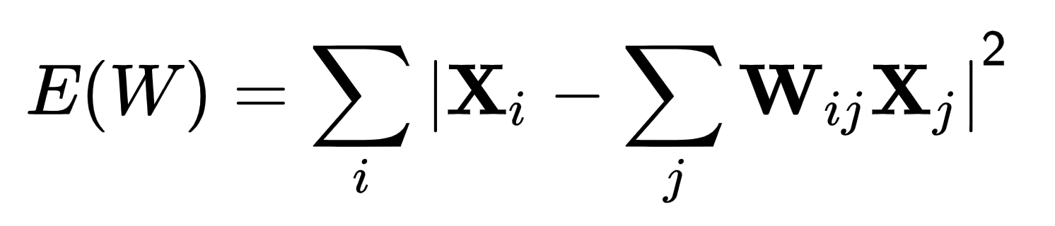
- This function is simply the sum of errors between each point $X_i$ and its reconstruction from its neighbors $X_j$.
## Mean Encoding
- https://towardsdatascience.com/why-you-should-try-mean-encoding-17057262cd0
- Encode the feature based on the **ratio of occurence of the positive class in the target variable**.
## Handy Tools
### Xverse
#### Overview
xverse (XuniVerse) is collection of transformers for feature engineering and feature selection
- https://github.com/Sundar0989/XuniVerse
- https://towardsdatascience.com/introducing-xverse-a-python-package-for-feature-selection-and-transformation-17193cdcd067
### feature-selector
#### Overview
Feature selector is a tool for dimensionality reduction of machine learning datasets.
- https://github.com/WillKoehrsen/feature-selector
- https://towardsdatascience.com/a-feature-selection-tool-for-machine-learning-in-python-b64dd23710f0
 Sign in with Wallet
Connect another wallet
Sign in with Wallet
Connect another wallet