# Machine Learning Note
## What is Machine Learning?
- https://towardsdatascience.com/practical-machine-learning-with-c-and-grt-a54857972434
> An approach to computing that enables programs to generate predictable output based on a given input **without** using explicitly defined logic.
>
- https://www.slideshare.net/tw_dsconf/ss-62245351
- https://www.youtube.com/watch?v=ZrEsLwCjdxY&t=18s

## Concept
### Entropy
- https://towardsdatascience.com/entropy-how-decision-trees-make-decisions-2946b9c18c8

### Underfitting, Just Right, and Overfitting

#### Prevent Overfitting
- https://medium.com/yottabytes/a-quick-guide-on-basic-regularization-methods-for-neural-networks-e10feb101328
- Methods
1. L1, L2 regularization
2. weight decay
3. dropout
4. batch normalization
5. data augmentation
6. early stopping

### Hyperparameter
- https://medium.com/mlait/hyperparameters-in-machine-learning-fa45ccec9f6c
- A hyperparameter is a parameter or a variable we need to set before applying a machine learning algorithm into a dataset.
- These parameters express "High Level" properties of the model such as its complexity ot how fast it should learn.
- Usually fixed before the actual training process begins.
- Two categories: optimizer and model hyperparameters

#### Optimizer Hyperparameters
- These are the variables or parameters related more to the optimization and training process then to model itself.
- They help you to tune or optimize your model before the actual training process starts so that you start at the right place in the training process.
- We here describe three of them:
- **Learning Rate**: a hyperparameter that controls how much we are adjusting the weights.
- For example, adjusting the weights of our neural network with respect to the gradient.
- **Mini-Batch Size**: a hyperparameter that has an effect on the resource requirements of the training and also impacts training speed and number of iterations.
- **Number of Training Iteration/Epochs**: it is a one complete pass through the training data.

#### Model Hyperparameters
- These are the variables which are more involved in the architecture or structure of the model.
- It defines your model complexity on the basis of:
- **Number of Layers**
- **Layers** is a general term that applies to a collection of 'nodes' operating together at a specific depth within a **neural network**.
- Different layers like input layer, hidden layer and output layer.
- **Hidden Units**: number of hidden layers in a neural network.
- The more complex the model (means more **hidden layers**), the more learning capacity the model will need.
- **Model Specific for parameters the architectures like RNN**
- Choosing a cell type like LSTM Cells, Vanilla RNN cells or GRU cells and how deep the model is.

### Backpropagation
https://medium.com/swlh/backpropagation-step-by-step-13f2b6c0b414
https://medium.com/@pdquant/all-the-backpropagation-derivatives-d5275f727f60

### Curse of Dimensionality
https://towardsdatascience.com/the-curse-of-dimensionality-minus-the-curse-of-jargon-520da109fc87
> In a nutshell, the curse of dimensionality is all about loneliness.

### MISC
#### Gradient Based Optimizations: Jacobians, Jababians & Hessians
https://medium.com/swlh/gradient-based-optimizations-jacobians-jababians-hessians-b7cbe62d662d
#### Matrix Decomposition & Algorithms
- https://medium.com/mlearning-ai/matrix-decomposition-and-algorithms-675339d8f48a
##### Why we need to study Decomposition?

> Decomposition is very important in algorithmic perspective in order to understand performance. In computation, these are required to consider time and space complexity to evaluate the performance. Decomposition methods are used to calculate determinant, upper and lower triangle matrices, matrix inversion, eigen values and eigen vectors, etc., to work on various types of matrices (symmetric, non-symmetric, square, non-square ). In a nutshell, decomposition helps us to write optimistic algorithms, and calculate Linear Algebra Object properties and various matrices.

## Feature Engineering
[Feature Engineering Note](/4AjdxBn1SUCPwAr4xP11YA)

## Loss Functions
### Label Smoothing
- https://medium.com/@lessw/label-smoothing-deep-learning-google-brain-explains-why-it-works-and-when-to-use-sota-tips-977733ef020

### Cross Entropy
- https://towardsdatascience.com/cross-entropy-for-dummies-5189303c7735
- Cross entropy is commonly used as a loss function for classification problems.
#### Entropy
- Claude Shannon formalised this intuition behind information in his seminal work on Information Theory.
- He defined information as:

I(x) = -log₂P(x) ..where P(x) is probability of occurrence of x

- Consider the following example. A bin contains 2 red, 3 green, and 4 blue balls. Now, instead of tossing a coin, I pick out one ball at random and give it to you.
- What is the expected amount of information you will receive every time I pick one ball?
- We model *picking* out a ball as a stochastic process represented by a random variable X.
- The entropy of X is then defined as the *expected value* of the information conveyed by an outcome in X.
- Using our above definition of information, we get:

P(red ball) = 2/9; I(red ball) = -log₂(2/9)
P(green ball) = 3/9; I(green ball) = -log₂(3/9)
P(blue ball) = 4/9; I(blue ball) = -log₂(4/9)
Entropy = E[I(all balls)] 
= -[(2/9)*log₂(2/9) + (3/9)*log₂(3/9) + (4/9)*log₂(4/9)]
= 1.53 bits.

:::info
Expected Value or Expectation of random variable X, written as E[X], is the average of all values of X weighted by the probability of their occurrence.
:::
- In other words, you can expect to get 1.53 bits of information on average every time I pick out a ball from the bin.
- Formally, the entropy H of a probability distribution of a random variable is defined as:
- The x~P in the above equation means that the values x takes are from the distribution P. In our example, P = (2 red, 3 green, 4 blue).

#### Cross Entropy
- Cross-entropy measures the relative entropy between two probability distributions over the same set of events.
- ntuitively, to calculate cross-entropy between P and Q, you simply calculate entropy for Q using probability weights from P. Formally:
- Let’s consider the same bin example with two bins:

Bin P = {2 red, 3 green, 4 blue}
Bin Q = {4 red, 4 green, 1 blue}
H(P, Q) = -[(2/9)*log₂(4/9) + (3/9)*log₂(4/9) + (4/9)*log₂(1/9)]

#### Cross-Entropy as Loss Function
- Instead of the contrived example above, let’s take a machine learning example where we use cross-entropy as a loss function.
- Suppose we build a classifier that predicts samples in three classes: A, B, C.
- Let P be the true label distribution and Q be the predicted label distribution. Suppose the true label of one particular sample is B and our classifier predicts probabilities for A, B, C as (0.15, 0.60, 0.25)
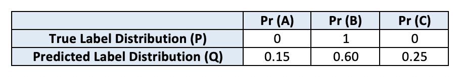
- Cross-entropy H(P, Q) will be:

H(P, Q) = -[0 * log₂(0.15) + 1 * log₂(0.6) + 0 * log₂(0.25)] = 0.736

- On the other hand, if our classifier is more confident and predicts probabilities as (0.05, 0.90, 0.05), we would get cross-entropy as 0.15, which is lower than the above example.

#### Relation to Maximum Likelihood
- For *classification problems*, using cross-entropy as a loss function **is equivalent to** maximising log likelihood.
- Consider the below case of binary classification where a, b, c, d represent probabilities:

H(True, Predicted)
= -[a*log(b) + c*log(d)]
= -[a*log(b) + (1-a)*log(1-b)]
= -[y*log(ŷ) + (1-y)*log(1-ŷ)]
..where y is true label and ŷ is predicted label

- This is the same equation for maximum likelihood estimation.

### Swish
https://medium.com/analytics-vidhya/swish-booting-relu-from-the-activation-function-throne-78f87e5ab6eb
- Like ReLU, Swish is bounded below but unbounded above. However, Switch is *smooth* (does not have sudden changes of motion or a vertex) unlike ReLU.
- In addition, Swish is *non-monotonic*, meaning that there is not always a sigularity and continually positive (or negative) derivative throughout the entire function.
#### Formula

Derivative

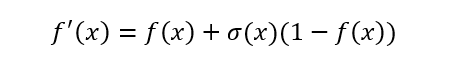
The first and second derivatives of Swish:
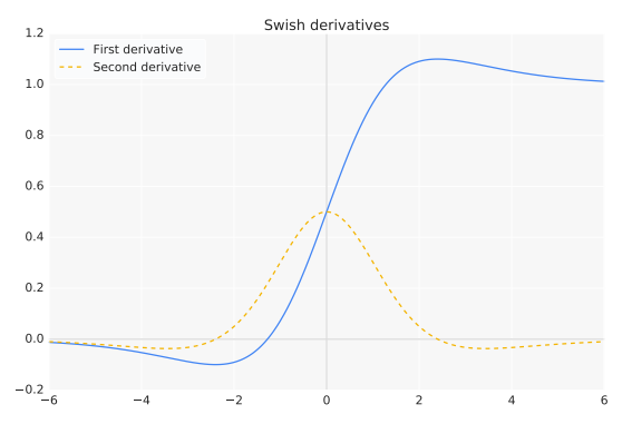
For inputs less than about 1.25, the derivative has a magnitude of less than 1.

### Why is my validation loss lower than my training loss?
https://medium.com/analytics-vidhya/deep-learning-why-is-my-validation-loss-lower-than-my-training-loss-5a7a5cf3fb2c
#### Reason #1: Regularization applied during training, but not during validation/testing
When training a DNN we often apply **regularization** to help our model:
1. **Obtain higher validation/testing accuracy**.
2. And ideally, to **generalize better**.

Regularization often **sacrifice training accuracy to improve validation/testing accuracy** -- in some cases that can lead to your validation loss lower than training los.

**Secondly, keep in mind that regularization such as dropout are *not* applied at validation/testing.**
#### Reason #2: Training loss is measured during each epoch while validation loss is measured after each epoch
Your training loss is continually reported over the course of an entire epoch; however, **validation are computed over the validation set *only once the current training epoch is complete*.**

This implies, on average, training loss are measured half an epoch earlier.

If you shift the training losses half an epoch to the left you'll see that the gaps between the training and losses values are much smaller.
#### Reason #3: The validation set may be easier than the training set (or there may be leaks)
Consider how your validation set was acquired:
1. Can you guarantee that the validation set was sampled from the same distribution as the training set?
2. Are you certain that the validation examples are just as challenging as your training images?
3. Can you assure there was no “data leakage” (i.e., training samples getting accidentally mixed in with validation/testing samples)?
4. Are you confident your code created the training, validation, and testing splits properly?

**Every single deep learning practitioner has made the above mistakes at least once in their career.**

Yes, it is embarrassing when it happens — but that’s the point — it does happen, so take the time now to investigate your code.

### multicollinearity
https://towardsdatascience.com/how-to-avoid-multicollinearity-in-categorical-data-46eb39d9cd0d
#### Definition
- Multicollinearity refers to a condition in which the **independent variables are correlated to each other**.
- Multicollinearity can cause problems when you fit the model and interpret the results.
- The variables of the dataset should be independent of each other to overdue the problem of multicollinearity.
#### Symptoms
- Getting very high standard errors for regression coefficients
- The overall model is significant, but none of the coefficients are significant
- Large changes in coefficients when adding predictors
- High Variance Inflation Factor (VIF) and Low Tolerance

#### Solutions
- PCA, etc.

## Metrics
### Train/Test Errors
Omitted because it is obvious.

### Receiver Operating Characteristic (ROC) Curve
https://towardsdatascience.com/classifying-rare-events-using-five-machine-learning-techniques-fab464573233
- ROC is a graphic representation showing how a classification model performs at all classification thresholds.
- We prefer a classifier that approaches to 1 quicker than others.
- ROC Curve plots two parameters -- True Positive Rate and False Positive Rate -- at different thresholds in the same graph:
> TPR (Recall) = TP / (TP + FN)
> FPR = FP / (TN + FP)
>

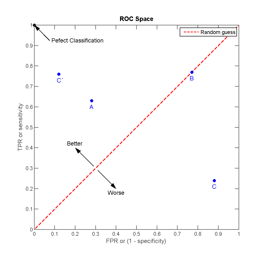
- To a large extent, ROC Curve does not only measure the level of classification accuracy but reaches a nice balance between TPR and FPR.
- This is quite desirable for rare events since we also want to reach a balance between the majority and minority cases.

### Area Under the Curve (AUC)
https://towardsdatascience.com/classifying-rare-events-using-five-machine-learning-techniques-fab464573233
- As name suggested, AUC is the area under the ROC curve.
- It is an arithmetic representation of the visual AUC curve.
- AUC provides an aggerated results of how classification perform across possible classification thresholds.

### Implementation from scratch
ROC Curve and AUC From Scratch in NumPy (Visualized!)
- https://towardsdatascience.com/roc-curve-and-auc-from-scratch-in-numpy-visualized-2612bb9459ab

## Activation Functions
### Famous Activation Funstions Plot Comparison
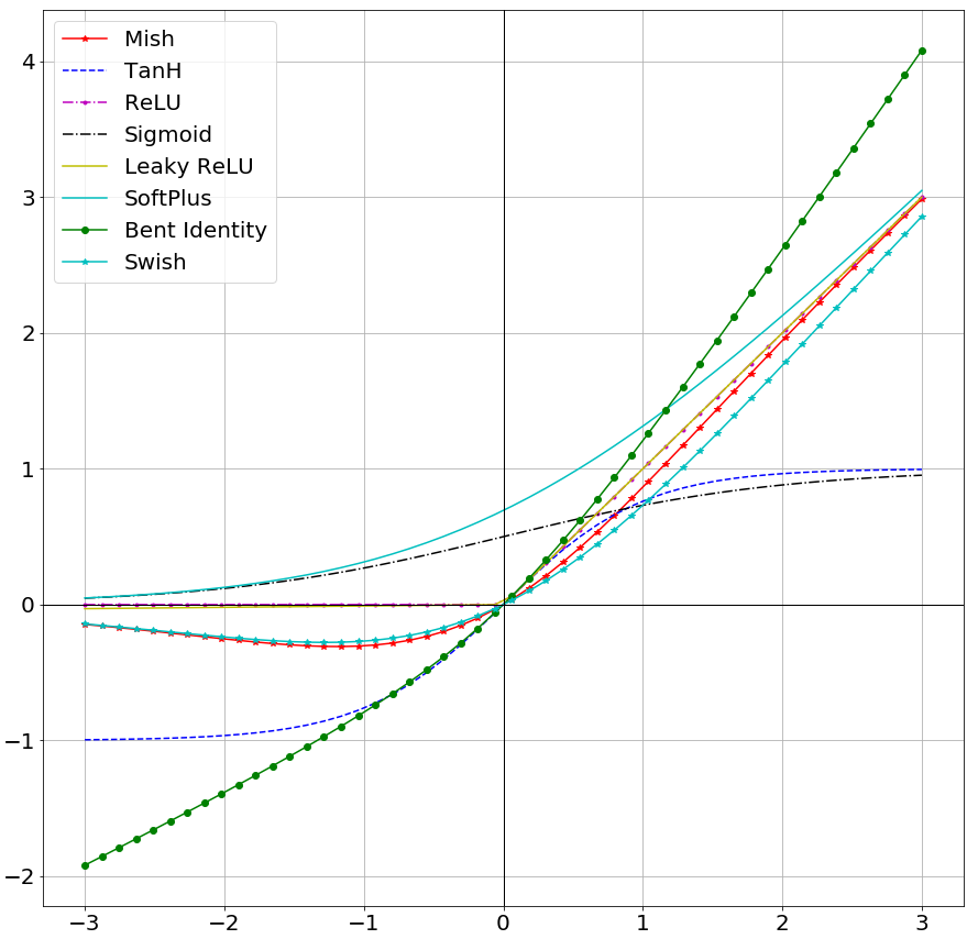
<center>Activation Function Plots</center>

### Swish
#### Paper
- https://arxiv.org/pdf/1710.05941v1.pdf
#### Overview
https://towardsdatascience.com/mish-8283934a72df
In 2017, Researchers at Google Brain, published a new paper where they proposed their novel activation function named Swish. Swish is a gated version of Sigmoid Activation Function, where the mathematical formala is: $f(x,\beta) = x * Sigmoid(x, \beta)$ [Often Swish is referred as SILU or simply Swish-1 when β=1]

Their results showcased a significant improvement in Top-1 Accuracy for ImageNet at 0.9% better than ReLU for Mobile NASNet-A and 0.7% for Inception ResNet v2.
### Mish
#### Overview
Mish: A Self Regularized Non-Monotonic Neural Activation Function
https://towardsdatascience.com/mish-8283934a72df
- Inspired from Google Brain's Paper -- [*Swish: A Self-Gated Activation Function*](https://arxiv.org/pdf/1710.05941v1.pdf), Mish is an easy to implement and intuitively simple activation function.
- Mathematically, *Mish* Activation Function is a modified Gated form of Softplu Activation Function.
- The Softplus Activation Function can be represented as:
<center>SoftPlus Activation Function</center>

- Thus *Mish* can be mathematically defined as:
<center>Mish Activation Function</center>
#### Source Code
- https://github.com/digantamisra98/Mish

## Model Explanation (Interpretation)
[Model Explanation](/XhfDAcMEQtWS0n3QVBWM5A)

## Data Augmentation
### Tools
- Imgaug
- https://towardsdatascience.com/data-augmentation-techniques-in-python-f216ef5eed69

## Ensemble Learning
- https://medium.com/earthcube-stories/boosting-object-detection-performance-through-ensembling-on-satellite-imagery-949e891dfb28
- A technique that aims to maximize the final detection performance by fusing individual detections.
- All ensemble learning methods rely on combinations of model variations in at least one of the three following spaces: *training data, model space*, and *prediction space*.

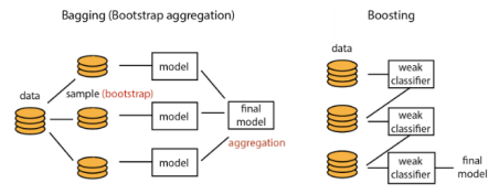
### Training Data
- **bagging** and **boosting**
- difference between bagging and boosting

### Model Space
- Several techniques have emerged to generate variations of the original model (called snapshots) during the training to substantially increase the performance.
- *Snapshot Ensembling*, *Fast Geometrical Ensembling*, and *Stochastic Weights Averaging*
- *Snapshot Ensembling (SSE)* cyclically modifies the learning rate so that the model reaches several local minima during the training.
- A snapshot is taken for each of the local minima and their predictions are fused.
- Nevertheless, this increases substantially the training time.
- Not suit to very large training sets.
- *Fast Geometrical Ensembling (FGE)* also modifies cyclically the learning rate to move the model along a low pass path in the weights space and generates snapshots with similar performance but different behaviors.
- It can thus be used as a fine-tuning and solves the training time issue of *SSE*.
- *Stochastic Weights Averaging (SWA)* is very close to *FGE*, but instead of fusing the predictions of the snapshots, the model weights are fused to generate a more robust unique model.
- So that the computation time at prediction is not impacted.
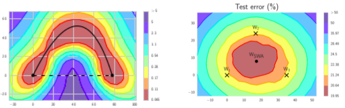
<center>Weights space — left: low-loss path of the FGE technique (source [4]), right: average of three snapshot weights resulting in the SWA weights (source [5])</center>

### Prediction Space
- *voting*
- benefit: ease to use in production
- drawback: using a low-performance individual model (even if very efficient on one specific type of the input data) will decrease the overall performance.
- *stacking*
- benefit: solve the issue of voting
- A new trained model and takes in input the predictions of the individual models, so even weak models can participate to increase the overall performance.
- drawback: the fusion model needs to be re-trained if one of the individual models is modified, so it's hard to use in production.
- *Test-time Augmentation (TTA)*
- It modifies the input image at prediction time (rotation, translation, intensity, etc.)
- promising and no need to any new training
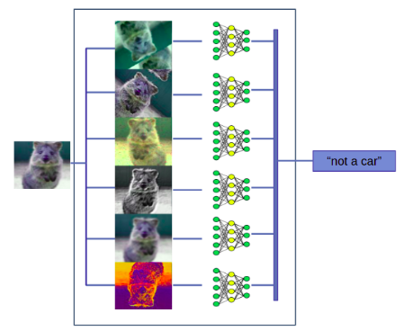
<center>Example of the Test-Time Augmentation (TTA) concept</center>

- *Bayesian dropout*
- It disables a set of randomly chosen neurons in the model.
- promising and no need to any new training

## Regressions
### Simple Linear Regression
- https://medium.com/sigmoid/linear-regression-from-scratch-with-python-5c33712a1cec
- https://github.com/sarvasvkulpati/LinearRegression
- Linear Regression is a method for approximating a linear relationship between two variables.
- All it really means is that it takes some input variable, like the age of a hous, and finds out how it's related to another variable, for example, the price it sells at.
- We use it when the data has a **linear relationship**, which means that when you plot the points on a graph, the data lies approximately in the shape of a straight line.
#### Goal
- The goal of linear regression is to find a line that best fits a set of data points.
#### Steps
1. Randomly initialize parameters for the hypothesis function.
2. Compute the mean square error (MSE).
3. Calculate the partial derivatives.
4. Update the parameters based on the derivatives and the learning rate.
5. Repeat from 2-4 until the error is minimized.
#### The Hypothesis Function
- The **linear equation** is the standard form that represents a straight line on a graph, where $m$ represents the **grident -- how steep the line is**, and $b$ represents the **y-intercept -- where the line crosses the y-axis**.
- You might remember this as one of the first equations you learned from school:
$$
y = mx + c
$$
- The Hypothesis function is the **exact** same function in the notation of Linear Regression.
$$
h_{\theta}(x) = \theta_{1}x+\theta_{0}
$$
- The two variable we can change -- $m$ and $b$ -- are represented as parameters $\theta_{1}$ and $\theta_{0}$.
#### The Error Function
- It calculates the total error of your line.
- We'll be using an error function called the Mean Square Error function, namely MSE, represented by the letter $J$.
$$
J(\theta_{0}, \theta_{1}) = \frac{1}{2}\sum_{i=1}^{m}(h_{\theta}(x_{i})-y_{i})^2
$$
- While it may look complex, what it's doing is actually quite simple:
1. To find out how "wrong" the line is, we need to find out how far it is from each points. To do this, we subtract the actual value $y_i$ from the predicted value $h_{\theta}(x_{i})$.
2. However, we don't want the error to be negative, so to make sure it's positive at all times, we square this value.
3. $m$ is the number of points in our dataset. We then repeat this subtraction and squaring for all $m$ points.
4. Finally, we divide the error by 2. This will help use later when we are updating our parameters.
- Now we have the value for how wrong our function is, we need to adjust the function to reduce this error.
#### Calculating Derivatives
- Our goal with linear regression is to find the line which best fits a set of data points. In other words, it's the line that's the least incorrect or has the lowest error.
- If we graphour parameters against the error, i.e. graphing the cost function, we'll find that it forms something similar to the graph below. At the lowest point of the graph, the error is at it's lowest, Finding this point is called **minimizing the cost function**.
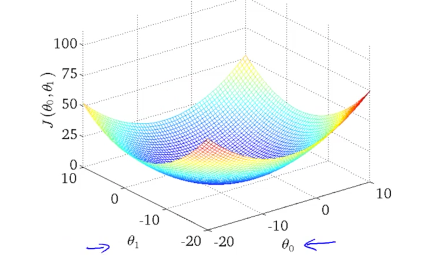
- To do this, we need to consider what happens at the bottom of the graph, or the gradient is zero.
- So **to minimize the cost function, we need to get the gradient to zero**.
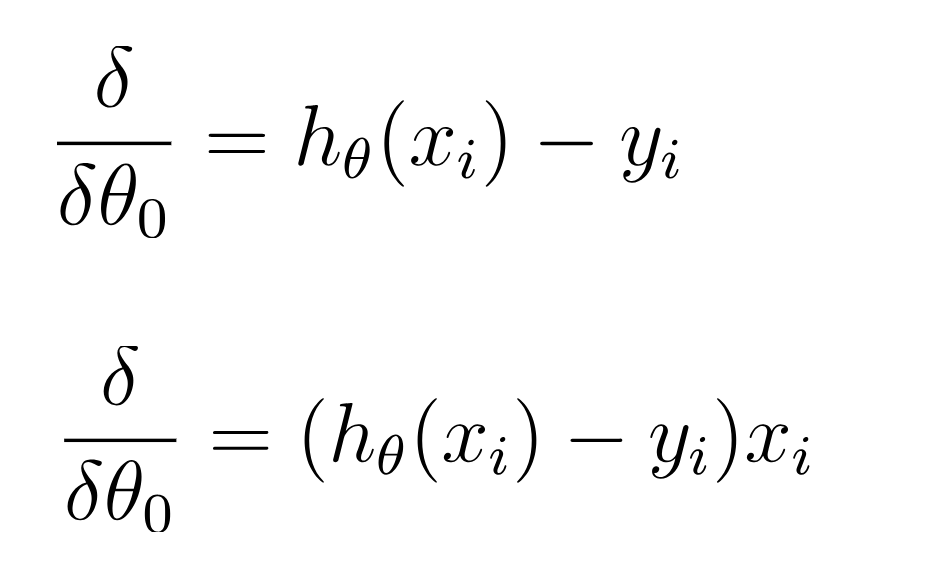
- The gradient is given by the derivative of the function, and the partial derivatives of the function are:
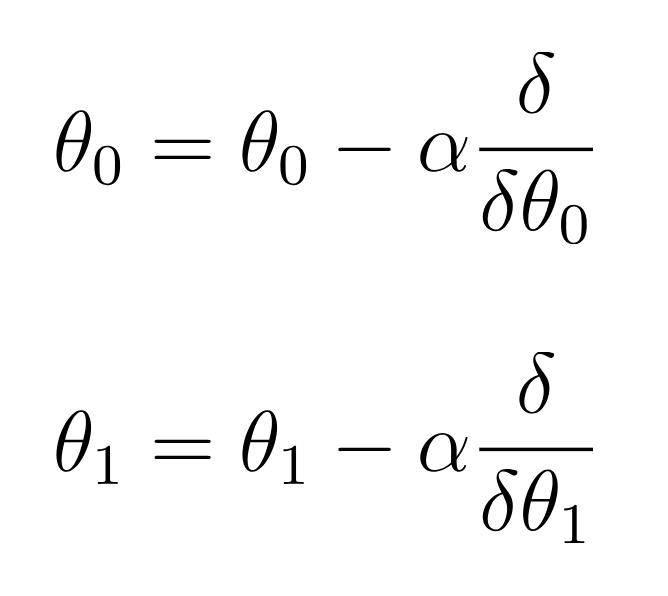
#### Updating the Parameters Based on the Learning Rate
- Now we need to update the parameters to reduce the graident. To do this, we use the graident update rule.
- **Alpha(α) is what we call the Learning Rate, which is a small number that allows the parameters to be updated by a small amount**.
- The learning rate helps guide the network to the lowest point on the curve by small amounts.
#### Minimizing the Cost Function
- Now we repeat these stpes -- checking the error, calculating the derivatives, and updaing the weights untils the error is as low as possible. This is called minimizing the cost function.
#### Why do we use “squared” errors and not higher powers or absolute values of the errors?
- https://towardsdatascience.com/introducing-linear-regression-least-squares-the-easy-way-3a8b38565560
1. With higher powers, an outlier’s error will amplify even more. As a result, the more the “best fit” line will get pulled towards the outlier and that would not be a best fit anymore.
2. Minimising a quadratic function is easy — you just differentiate it and set the derivatives to zero, which results in a linear equation — which we have centuries of tricks to help us solve.

### Ridge Regression
https://towardsdatascience.com/ridge-regression-python-example-f015345d936b
- Ridge Regression is almost identical to Linear Regression except that we introduce a small amount of bias.

### Isotonic Regression
- https://towardsdatascience.com/isotonic-regression-is-the-coolest-machine-learning-model-you-might-not-have-heard-of-3ce14afc6d1e
- Isotonic regression is a free-form **linear** model that can be fit to predict sequences of observations.
- **Must not be non-decreasing**.
- The reason is that an isotonic function is a monotonic function.
- It uses an interesting concept called "Order Theory".
- Order Theory deals with the idea of partially ordered and pre-ordered sets as a generalization of real numbers.
- weight least squares

### Logistic Regression
- We take the output of the linear function and squash the value within the range of [0,1] using the **sigmoid function** (logistic function).
- Typically, if the squashed value is greater than a threshold value we assign it a label 1, else we assign it a label 0.
- This justifies the name "logistic regression".
- Note that the difference between logistic and linear regression is that Logistic regression gives you a discrete outcome but linear regression gives a **continuous outcome**.
- https://towardsdatascience.com/support-vector-machine-vs-logistic-regression-94cc2975433f
- https://towardsdatascience.com/introduction-to-logistic-regression-66248243c148

#### PyTorch Implementation
- https://medium.com/dair-ai/implementing-a-logistic-regression-model-from-scratch-with-pytorch-24ea062cd856

## Naive Bayes
### tutorial
- https://www.analyticsvidhya.com/blog/2017/09/naive-bayes-explained/

## Hidden Markov Model (HMM)
- https://medium.com/ai-academy-taiwan/hidden-markov-model-part-1-d80d56811c2a

## SVM (Support Vector Machine)
- https://towardsdatascience.com/support-vector-machine-vs-logistic-regression-94cc2975433f
- It is an algorithm to find the hyperplane that has maximum margin in an N-dimentional space (N -- the number of features) that distinctly classifies the data points.
- Support vectors are data points that tare closer to the hyperplane and influence the position and orientation of the hyperplane.
- Using these support vectors, we maximize the margin of the classifier.
- Deleting the support vectors will change the position of the hyperplane.
- https://towardsdatascience.com/understanding-support-vector-machine-part-2-kernel-trick-mercers-theorem-e1e6848c6c4d
- Mapping data points from low dimensional space to a higher dimensional space can make it possible to apply SVM even for non-linear data sample.
- We don’t need to know the mapping function itself, as long as we know the Kernel function ; ***Kernel Trick***
- Condition for a function to be considered as kernel function; *Positive semi-definite Gram matrix*.
- Types of kernels that are used most.
- How the tuning parameter gamma can lead to over fitting or bias in RBF kernel.
### Kernel Trick
- The idea is mapping the non-linear separable data-set into a higher dimensional space where we can find a hyperplane that can separate the samples.

### Visualizing SVM with Python
- https://medium.com/swlh/visualizing-svm-with-python-4b4b238a7a92

## Decision Tree Based
[Decision Tree Based Note](/3_7a89IuSC6_2Caq-1c4vg)

## Unsupervised Methods
### Overview
- https://towardsdatascience.com/clustering-for-data-nerds-ebbfb7ed4090
### kNN
https://towardsdatascience.com/beginners-guide-to-k-nearest-neighbors-in-r-from-zero-to-hero-d92cd4074bdb
- To decide the label ofr new observations, we look at the closest neighbors.
- To choose the nearest neighbors, we have to define what distance is.
- For categorical data, there are Hamming Distance and Edit Distance.

## Neural Network Based
### CNN
Nov. 29th, 2019 added: Too many contents so moved to [here](https://hackmd.io/cOjAq3HFQJiTANiMc8ZFCA?view)

### RNN
[RNN note](/OecNgNUHSROPdeVFbXmUKA)

### GNN
- https://towardsdatascience.com/graph-neural-networks-an-overview-dfd363b6ef87
- https://arxiv.org/pdf/1901.00596.pdf
- https://www.youtube.com/watch?v=L7-MkgS-ue4

#### Intro
- https://distill.pub/2021/gnn-intro/

#### Graph Convolution Types
##### Spectral
operates on Laplacian matrix and requires all the data-points to be present.
- not scalable to large graphs
- only capable of transductive learning

##### Spatial
Learns a set of aggregators or mechanisms that are shared across all the neighborhoods.
- computationally efficient -- scalable to large graphs
- readily applicable to both transductive and inductive problems

##### GraphSAGE (spatial)
uses either non-parametric aggregators (mean/max pooling), or parametric aggregators (LSTM) to aggregate neighborhood infomation

##### GAT (spatial)
uses multi-head attention mechanisms to aggregate neighborhood information

### GAN
- https://towardsdatascience.com/understanding-and-optimizing-gans-going-back-to-first-principles-e5df8835ae18
- https://towardsdatascience.com/must-read-papers-on-gans-b665bbae3317

#### DCGAN
- https://towardsdatascience.com/dcgans-deep-convolutional-generative-adversarial-networks-c7f392c2c8f8
- https://github.com/GANs-in-Action/gans-in-action/blob/master/chapter-3/Chapter_3_GAN.ipynb

#### SeqGAN
##### Overview
SeqGAN: GANs for sequence generation
https://medium.com/ai-club-iiitb/seqgan-gans-for-sequence-generation-5c74a84cd230

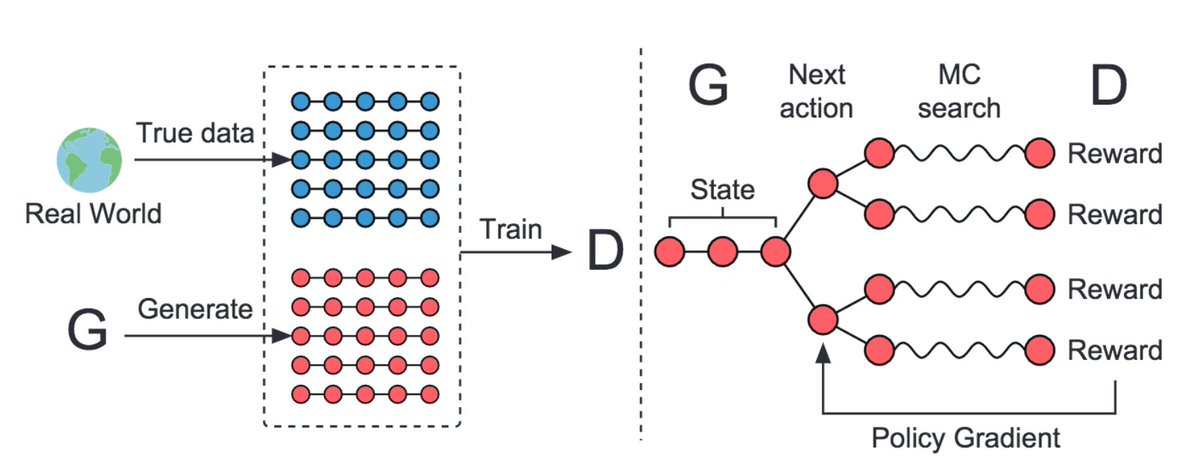
<center>The architecture diagram for SeqGAN</center>

- In SeqGANs, the generator is treated as an **RL agent**.
- **State**: Tokens generated so far
- **Action**: Next tokens to be enerated
- **Reward**: Feedback given to guide G by D on evaluating the generated sequence
- As the gradients cannot pass back to G due to discrete outputs, G is regarded as a stochastic parametrized policy. The policy is trained using policy gradient.
- The discriminator value is the probability of the generated sequence being real.

##### Procedure
1. Use G to generate a sequence Y(1:T)
2. For each time step t, calculate the action-value function reward
3. Update the generator parameters via policy gradient
4. Repeat 1-3 for g-steps
5. Using current G, generate negative samples
6. Combine above negative samples with positivie samples from training set
7. Train D using above combined samples
8. Repeat 5-7 for d-steps

##### Background
- When it comes to to sequential data (text, speech, etc.), there are some limitations in applying the exact same concepts. These limitations arise mainly due to the sequential and discrete nature of the data.
- Typically text tokens (say, words) are represented by an "embedding-vector" of real-values. **These values, though composed of continuous real-values, are discrete!**
- For Example, the word "computer" is represented bythe real-value vector v = [0.11143, -0.97712, 0.445216 ….., 0.7221240]. Now, v + 0.08 is another vector which need not necessarily represent some word in the vocabulary.
- ***So utilising the gradient of the loss from Discriminator with respect to the outputs of Generator to guide its parameters makes little sense.*** Thus the discreteness of text tokens is a hindrance to the usage of vanilla GANs for sequence generation.
- Secondly, Discriminator can only classify and give the loss for **an entire sequence**. For partial sequence, it cannot provide any feedback on how good the partial sequence is and what the future score of the entire sequence might be.

#### Training Techniques
- https://towardsdatascience.com/10-lessons-i-learned-training-generative-adversarial-networks-gans-for-a-year-c9071159628
1. Stability and Capacity
2. Early Stopping
3. Loss Funtion Selection
4. Balancing Generator and Discriminator Weight Updates
5. Mode Collapse and Learning Rate
6. Adding Noise
7. Label Smoothing
8. Multi-Scale Gradient
9. TTUR (Two Time-scale Update Rule)
10. Spectral Normalization

#### Generative Query Network
https://medium.com/swlh/generative-query-network-6e26423e3ac
- The GQN is mainly comprised of three architectures: a representation, a generation, and an auxiliary inference architecture.

### BERT
- https://medium.com/%E6%88%91%E5%B0%B1%E5%95%8F%E4%B8%80%E5%8F%A5-%E6%80%8E%E9%BA%BC%E5%AF%AB/nlp-model-google-bert-149c02c24b6a

### Embeddings
#### Introduction
- https://towardsdatascience.com/neural-network-embeddings-explained-4d028e6f0526

#### Entity Embeddings
Enhancing categorical features with Entity Embeddings
https://medium.com/@bressan/enhancing-categorical-features-with-entity-embeddings-e6850a5e34ff
- Source code: https://github.com/rodrigobressan/entity_embeddings_categorical
- Here's the question: does treating categorical value as being completely different from on another, such as when using One-Hot Encoding, really makes sense?
- With the above question, we can then proceed to the adoption of a technique popularly known in the NLP field as **Entity Embeddings**, which allows us to map a given feature set into a new one with a smaller number of dimensions.
- The usage of Entity Embeddings is based on the process of training Neural Network with the categorical data, with the purpose to retrieve the weights of the Embedding layers.
- This allows us to have a **more significant** input when compared to a single One-Hot-Encoding approach.
- Entity Embeddings also mitigate two major problems:
- No need to have a domain expert so that we can avoid the feature engineering step.
- Shrinkage on computing resources, once we're no longer encoding our possible categorical values with One-Hot-Encoding.

### Transformer
- https://mp.weixin.qq.com/s/ZlUWSj_iYNm7qkNF9rm2Xw?fbclid=IwAR0eqRpli_l9EohcuKNFrqqf-QMs3fvmVbp2Vry4B_ulrcRzCBy4OMTpl7s

#### Visual Transformers
paper
https://arxiv.org/abs/2006.03677

Visual Transformers: A New Computer Vision Paradigm
https://medium.com/swlh/visual-transformers-a-new-computer-vision-paradigm-aa78c2a2ccf2

### Attention
- https://arxiv.org/abs/1502.03044
- https://medium.com/swlh/attention-please-forget-about-recurrent-neural-networks-8d8c9047e117
- https://www.zhihu.com/question/36591394
- https://medium.com/@bgg/seq2seq-pay-attention-to-self-attention-part-1-d332e85e9aad
#### Self-Attention
https://towardsdatascience.com/illustrated-self-attention-2d627e33b20a

### Autoencoder
> An autoencoder is a special type of nueral network with a bottleneck layer, namely **latent representation**, for dimensionality reduction:
> $$z = f(x)$$
> $$x'=g(z)=g(f(x))\approx x,$$
> where $x$ is the original input, $z$ is the latent representation, $x'$ is the reconstructed input, and function $f$ and $g$ are the encoder and decoder respectively.
> The aim is to minimize the difference between the reconstructed output $g(f(x))$ and the original $x$, so that we know the latent representation $f(x)$ of the smaller size actually preserves enough features for reconstruction.
> https://towardsdatascience.com/building-a-convolutional-vae-in-pytorch-a0f54c947f71
#### Tied Weight Autoencoder
- https://medium.com/@lmayrandprovencher/building-an-autoencoder-with-tied-weights-in-keras-c4a559c529a2

#### VAE (Variation AudoEncoder)
> There is a question: how audoencoder can be altered for content generation. And this is the idea where the 'vairation' takes place.
> When we regualarize an autoencoder so that its latent representation is not overfitted to a single data, we can perform random sampling from the latent space, making our autoencoder 'variational'.
> To do so, we incorporate the idea of KL divergence for our loss function design.
> https://towardsdatascience.com/building-a-convolutional-vae-in-pytorch-a0f54c947f71

### Capsule Networks
#### Intro
https://medium.com/analytics-vidhya/introduction-to-capsule-networks-66ebcdde4837

### Normalization
https://towardsdatascience.com/difference-between-local-response-normalization-and-batch-normalization-272308c034ac
#### Why normalization
- Normalization has become a vital of DNN because of the unbounded nature of certain activation functions such as ReLU, ELU, etc.
- To limit the unbounded activation from increasing the output layer values, normalization is used just before the activation function.

#### Local Response Normalization (LRN)
- Introduced by AlexNet.
- To encourage *lateral inhibition*.
- It is a concept in Neurobiology which refers to the capacity of a neuron to reduce the activity of its neighbors. ([reference](https://www.learnopencv.com/batch-normalization-in-deep-networks/))
- In DNN, the purpose of this lateral inhibition is to carry out local contrast enhancement so that locally maximum pixels value are used as excitation for next layers.
- ++LRN is a **non-trainable layer** that square-normalizes the pixel values in a feature map in a within a local neighborhood.++
- There are two types of LRN based on the neightborhood defined and can seen in the figure below.

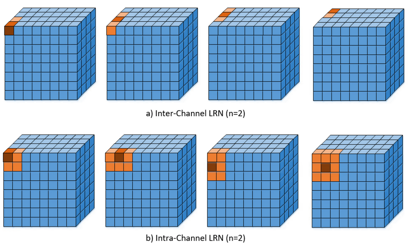
##### Inter-Channel LRN
- Originally what the AlexNet paper used.
- The neighborhood defined is **across the channel**.
- For each (x,y) position, the normalization is carried out in the depth dimension and is given by the following formula
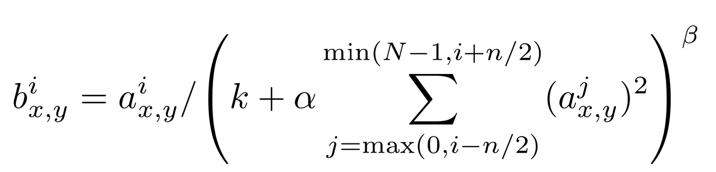
Where $i$ indicates the output of filter $i$, *a(x,y)*, *b(x,y)* the pixel values at *(x,y)* position before and after normalization respectively and N is the total number of channels.
- The constants (k,α,β,n) are hyper-parameters. k is used to avoid any singularities (division by zero), α is used as a normalization constant, while β is contrast constant. The constant n is used to define the neighborhood length i.e. how many consecutive pixel values need to be considered while carrying out the normalization.
- The case of (k,α, β, n)=(0,1,1,N) is the standard normalization). In the figure above n is taken to be to 2 while N=4.
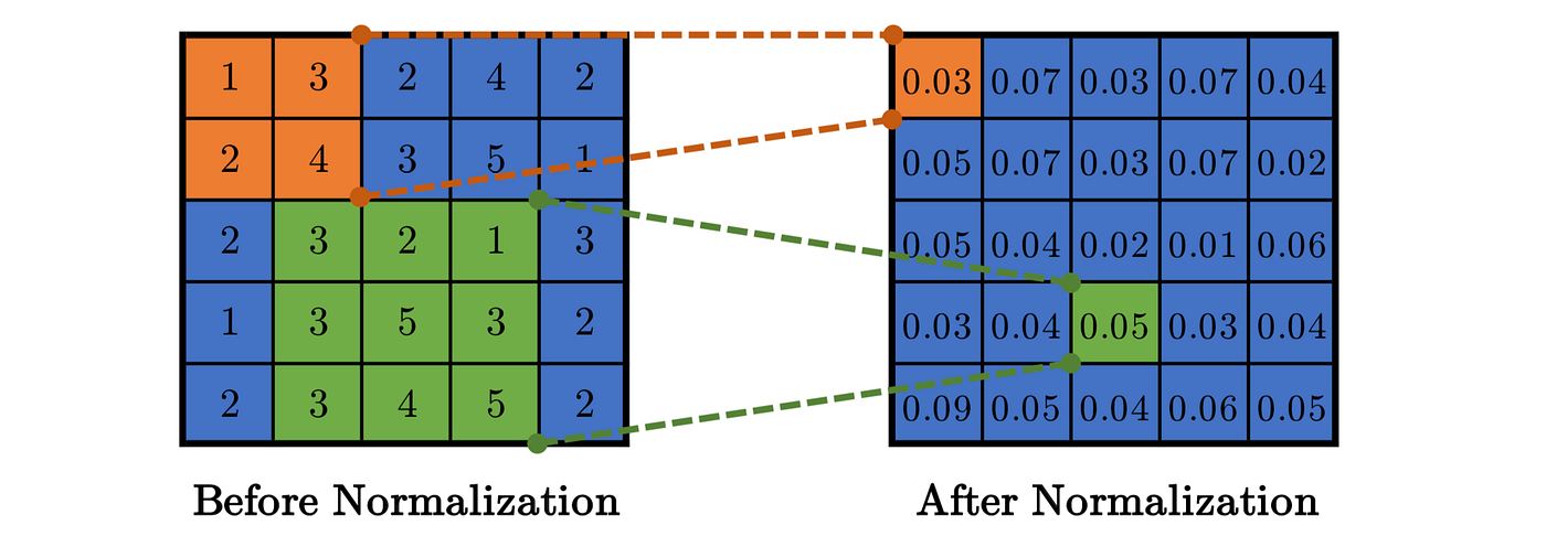
- Let's have a look at an example of Inter-channel LRN. Consider the following figure
Different colors denote different channels and hence N=4. Lets take the hyper-parameters to be (k,α, β, n)=(0,1,1,2). The value of n=2 means that while calculating the normalized value at position (i,x,y), we consider the values at the same position for the previous and next filter i.e (i-1, x, y) and (i+1, x, y). For (i,x,y)=(0,0,0) we have value(i,x,y)=1, value(i-1,x,y) doesn’t exist and value(i+,x,y)=1. Hence normalized_value(i,x,y) = 1/(1²+1²) = 0.5 and can be seen in the lower part of the figure above. The rest of the normalized values are calculated in a similar way.

##### Intra-Channel LRN
- The neighborhood is extended within the same channel only as it can seen.
- The formula is given by
where (W,H) are the width and height of the feature map (for example in the figure above (W,H) = (8,8)).

##### Difference Inter and Intra-Channel LRN
- The only difference between Inter and Intra Channel LRN is the neighborhood for normalization.
- In Intra-channel LRN, a 2D neighborhood is defined (as opposed to 1D neighborhood in Inter Channel) around the pixel under-consideration.
- As an example, the figure below shows the Intra-Channel normalization on a 5x5 feature map with n=2 (i.e. 2D neighborhood of size (n+1)x(n+1) centered at (x,y)).

#### Batch Normalization
- ++Batch Normalization (BN) is a **trainable layer** normally used for addressing the issues of **Internal Covariate Shift (ICF)**.++
- ICF arises due to the changing distribution of the hidden neurons/activation.
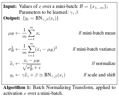
- In batch normalization, the output of hidden neurons is processed in the following manner before being fed to the activation function.
1. Normalize the entire batch B to be zero mean and unit variance
- Calculate the mean of the entire mini-batch output: u_B
- Calculate variance of the entire mini-batch output: sigma_B
- Normalize the mini-batch by subtracting the mean and dividing with variance
2. Introduce two trainable parameters (Gamma: scale_variable and Beta: shift_variable) to scale and shift the normalized mini-batch output
3. Feed this scaled and shifted normalized mini-batch to activation function.

The BN algorithm can be seen in the figure below.
- The normalization is carried out for each pixel across all the activations in a batch.
- Consider the figure below. Let us assume we have a mini-batch of size 3.
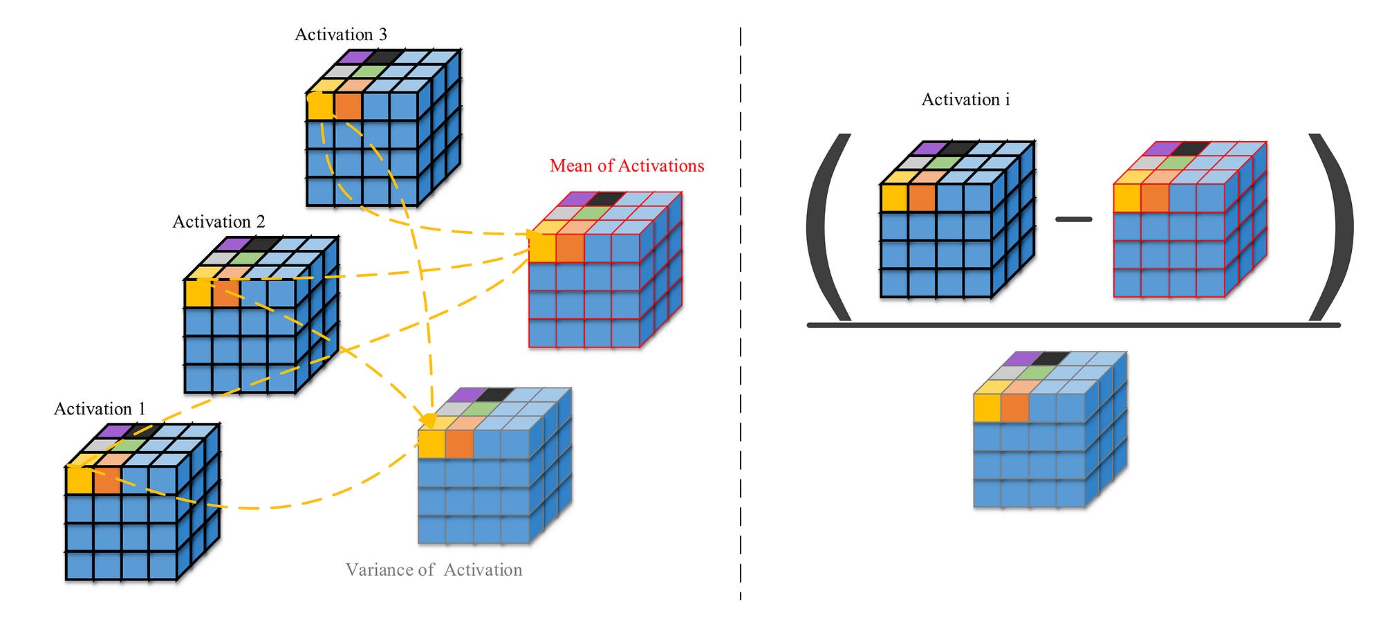
- A hidden layer produces an activation of size (C,H,W) = (4,4,4). Since the batch size is 3, we will have 3 of such activations.
- Now for each pixel in the activation (i.e. for each 4x4x4=64 pixel) we will normalize it by finding the mean and variance of this pixel position in all the activations as shown in the left part of the figure below.
- Once the mean and variance is found, we will subtract the mean from each of the activations and divide it with the variance.
- The right part of the figure below depicts this. The subtraction and division is carried out point-wise.

#### Comparison
- LRN v.s. BN

## MISC
- https://medium.com/jameslearningnote
- https://cnbeining.github.io/deep-learning-with-python-cn/3-multi-layer-perceptrons/ch9-use-keras-models-with-scikit-learn-for-general-machine-learning.html
- https://www.kaggle.com/mgiraygokirmak/keras-cnn-multi-model-ensemble-with-voting/notebook
- https://blog.slavv.com/37-reasons-why-your-neural-network-is-not-working-4020854bd607
- https://ithelp.ithome.com.tw/users/20129198/ironman/3001?fbclid=IwAR3tCueXmeVv7bwMAS74zS3-wBStejlrV_vsedO_dniO9h8nQ3Fp0P1TDeg

### 5 Ways to Detect Outliers/Anomalies That Every Data Scientist Should Know (Python Code)
- https://towardsdatascience.com/5-ways-to-detect-outliers-that-every-data-scientist-should-know-python-code-70a54335a623
1. Standard Deviation
2. Boxplots
3. DBScan Clustering
4. Isolation Forest
5. Robust Random Cut Forest

### How To Fine Tune Your Machine Learning Models To Improve Forecasting Accuracy?
https://medium.com/fintechexplained/how-to-fine-tune-your-machine-learning-models-to-improve-forecasting-accuracy-e18e67e58898

### How to Grid Search Hyperparameters for Deep Learning Models in Python With Keras
https://machinelearningmastery.com/grid-search-hyperparameters-deep-learning-models-python-keras/

### Multi-Class classification with Sci-kit learn & XGBoost: A case study using Brainwave data
https://medium.com/free-code-camp/multi-class-classification-with-sci-kit-learn-xgboost-a-case-study-using-brainwave-data-363d7fca5f69

### The Problem Of Overfitting And How To Resolve It
- https://medium.com/fintechexplained/the-problem-of-overfitting-and-how-to-resolve-it-1eb9456b1dfd

### How to Grid Search Hyperparameters for Deep Learning Models in Python With Keras
https://machinelearningmastery.com/grid-search-hyperparameters-deep-learning-models-python-keras/

### GridSearchCV with keras
https://www.kaggle.com/shujunge/gridsearchcv-with-keras

### 深度学习超参调优技巧
http://yangguang2009.github.io/2017/01/08/deeplearning/grid-search-hyperparameters-for-deep-learning/

### ROC and PR Curves
- https://machinelearningmastery.com/roc-curves-and-precision-recall-curves-for-classification-in-python/
- http://www.fullstackdevel.com/computer-tec/data-mining-machine-learning/501.html
- https://www.datascienceblog.net/post/machine-learning/interpreting-roc-curves-auc/

### Object detection - how to annotate negative samples
- https://stats.stackexchange.com/questions/315748/object-detection-how-to-annotate-negative-samples
- Short answer:
You don't need negative samples to train your model. Focus on improving your model.

### A Keras Pipeline for Image Segmentation
- https://towardsdatascience.com/a-keras-pipeline-for-image-segmentation-part-1-6515a421157d
- dataset list generator

### 7 Tips for Dealing With Small Data
- https://www.kdnuggets.com/2019/07/7-tips-dealing-small-data.html?fbclid=IwAR39Sl2_Vsy1reWm5f9FUrZKBZbgdCwGyo_xuyLMPq2IVuhlBatPpIqbDV4
1. Realize that your model won’t generalize that well.
2. Build good data infrastructure.
3. Do some data augmentation.
4. Generate some synthetic data.
5. Beware of lucky splits.
6. Use transfer learning.
7. Try an ensemble of “weak learners”.

### PyTorch Hooks to Print Each Layer Result
https://towardsdatascience.com/the-one-pytorch-trick-which-you-should-know-2d5e9c1da2ca
https://github.com/cosmic-cortex/pytorch-hooks-tutorial/blob/master/hooks.ipynb

### Optimizing object detection — Fusing & Filtering predicted boxes
https://towardsdatascience.com/wbf-optimizing-object-detection-fusing-filtering-predicted-boxes-7dc5c02ca6d3
1. Non-maximum suppression (NMS)
2. Soft-NMS
3. Weighted Boxes Fusion (WBF)

### 物件偵測模型如何輕量化？中華電信研究院分享自家3秘訣
https://www.ithome.com.tw/news/143462

## Handy Tools
### FasiAI-like stuffs
#### WEKA
- https://medium.com/datadriveninvestor/simplifying-machine-learning-using-weka-3df458fd2c6f
- http://blog.pulipuli.info/2017/04/auto-weka-automatic-model-selection-and.html

#### Ludwig
- Ludwig is a toolbox built on top of TensorFlow that allows to train and test deep learning models without the need to write code.
- https://github.com/uber/ludwig
- https://medium.com/gowombat/first-impressions-about-ubers-ludwig-a-simple-machine-learning-tool-or-not-714962bbbedc

### TFRecord
- https://medium.com/mostly-ai/tensorflow-records-what-they-are-and-how-to-use-them-c46bc4bbb564
- https://gist.github.com/tgamauf/5eb04f59becc045c88cba29fcd168d24#file-write_tfrecord_with_example-ipynb
- https://gist.github.com/tgamauf/ab5efb632bca8594fb39940d0641dc84#file-write_tfrecord_with_sequenceexample-ipynb

### Wandb
- https://wandb.ai/site
- https://zhuanlan.zhihu.com/p/342300434
- https://yanwei-liu.medium.com/wandb-weights-and-biases-a-better-choice-over-tensorboard-6c75b5f972b1

### AutoGAN
- https://towardsdatascience.com/automatically-finding-the-best-neural-network-for-your-gan-c0b97a5949f2

### Data Annotation
#### dhSegment
https://github.com/dhlab-epfl/dhSegment

### Data Augmentation
#### Albumentations
- https://github.com/albu/albumentations?source=post_page---------------------------

### Explainable AI
- https://medium.com/trustableai/%E5%AE%83%E6%98%AF%E6%80%8E%E9%BA%BC%E7%9F%A5%E9%81%93%E7%9A%84-%E8%A7%A3%E9%87%8B%E6%B7%B1%E5%BA%A6%E5%AD%B8%E7%BF%92%E6%A8%A1%E5%9E%8B-f18f57d18d4f
- LIME
- https://github.com/marcotcr/lime
- LRF
- heatmapping.org
- https://towardsdatascience.com/visual-interpretability-for-convolutional-neural-networks-2453856210ce

#### Keract
- https://github.com/philipperemy/keract
- example
- https://github.com/tirthajyoti/Deep-learning-with-Python/blob/master/Notebooks/Keract-activation.ipynb

### SHAP
- A game theoretic approach to explain the output of any machine learning model.

#### Source Code
- https://github.com/slundberg/shap

#### Document
- https://shap.readthedocs.io/en/latest/

#### Example
- https://towardsdatascience.com/explain-any-models-with-the-shap-values-use-the-kernelexplainer-79de9464897a

### Auto Optimizer
#### optuna
https://github.com/optuna/optuna
https://optuna.org/

### AutoML
#### AutoML with GitHub Actions
https://towardsdatascience.com/github-is-the-best-automl-you-will-ever-need-5331f671f105
https://github.com/pycaret/pycaret-git-actions
* Use GitHub Actions for AutoML to find the best model for free!

### Model Deployment
#### cortex
- https://github.com/cortexlabs/cortex
- https://towardsdatascience.com/how-to-deploy-onnx-models-in-production-60bd6abfd3ae

#### Anvil (Full Stack Web App)
https://anvil.works/
https://towardsdatascience.com/an-introduction-to-anvil-full-stack-web-apps-with-nothing-by-python-cbab06392d13

### Visualization
#### Tensorboard
- https://towardsdatascience.com/semantic-segmentation-visualization-of-learning-progress-by-tensorboard-7272fd5b6b50

#### CppFlow
- https://github.com/serizba/cppflow

#### ml-visuals
https://github.com/dair-ai/ml-visuals

### Visualized Model Maker
#### KNIME Analytics Platform
- https://towardsdatascience.com/knime-desktop-the-killer-app-for-machine-learning-cb07dbef1375

#### Tools-to-Design-or-Visualize-Architecture-of-Neural-Network
- https://github.com/ashishpatel26/Tools-to-Design-or-Visualize-Architecture-of-Neural-Network

### MISC
#### mlflow
- https://github.com/mlflow/mlflow
- https://medium.com/analytics-vidhya/tracking-deep-learning-experiments-using-keras-mlflow-and-mongodb-732fc771266c

## Framework Related
### Keras
#### Tutorial
https://ithelp.ithome.com.tw/2020-12th-ironman/articles/3128?sc=iThomeR
#### Callbacks
- https://medium.com/towards-artificial-intelligence/keras-callbacks-explained-in-three-minutes-846a43b44a16
- EarlyStopping
- ModelCheckpoint
- LearningRateScheduler
- History
- BaseLogger
- TensorBoard

#### Pruning
##### Keras-surgeon
- https://github.com/BenWhetton/keras-surgeon
- https://medium.com/@anuj_shah/model-pruning-in-keras-with-keras-surgeon-e8e6ff439c07?

### Gesture Recognition Toolkit (GRT)
- http://www.nickgillian.com/wiki/pmwiki.php/GRT/GestureRecognitionToolkit
- github
- https://github.com/nickgillian/grt

### PyTorch
[PyTorch Note](/4auyPeBjS-mftrt9wFuyOw)

### TensorFlow
[TensorFlow](/VjJtXwpNSLq6D2Ts3tLjNA)

### Xnor.ai
- https://medium.com/free-code-camp/perf-machine-learning-on-rasp-pi-51101d03dba2
- https://www.xnor.ai/
- A proprietary framework that reconfigures your model to run efficiently on smaller hardware.
- Xnor’s binary logic shrinks 32-bit floats to 1-bit operations, allowing you to optimize deep learning models for simple devices.

## NLP Related
[NLP Note](/f-QH6lIMRFSECnSSWprOvA)

## Reinforcement Learning
- https://medium.com/datadriveninvestor/how-to-implement-a-reinforcement-learning-library-from-scratch-a-deep-dive-into-reinforce-jl-d1ec2a239924
> ... a declarative way to teach machines certain behaviours. You specify some high-level reward functions like winning at Chess or Go and via self-play, they can beat human world champions at those games.

- https://github.com/zhoubolei/introRL

## knowledge distillation
https://towardsdatascience.com/knowledge-distillation-and-the-concept-of-dark-knowledge-8b7aed8014ac
### Benefit
- Get a lighter model.
- Less compute requirements and superior performance.
- Better accuracy than stand-alone model.
- Can be used even when there is lesser training data available for the student model. It is enough to have a well trained teacher.

### Difference between transfer learning
- In transfer learning, the weights are transferred from a pre-trained network to a new network and the pre-trained network should exactly match the new network architecture. What this means is that the new network is essentially as deep and complex as the pre-trained network.
- However, the objective of knowledge distillation is different. The aim is not to transfer weights but to transfer the generalizations of a complex model to a much lighter model.

### Terminology
- teacher-student network
- concept of temperature in softmax activation
- dark knowledge
- softened probabilities

### Assesment
https://arxiv.org/abs/1910.01348

## Dark Knowledge
When Does Label Smoothing Help?
https://medium.com/@nainaakash012/when-does-label-smoothing-help-89654ec75326

## Post-Training Optimization
Post-Training Optimization Techniques
- https://medium.com/@edgeneural.ai/post-training-optimization-techniques-6f428c16ec89
- hardware level
- software level
- algorithm level

## Applications
### Overview
https://arxiv.org/pdf/2009.05673.pdf
https://github.com/jeffheaton/t81_558_deep_learning
### Edge Computing
#### Simple Neural Network on MCUs
- https://medium.com/hacksters-blog/simple-neural-network-on-mcus-a7cbd3dc108c

### Lidar 3d Object Detection Methods
https://towardsdatascience.com/lidar-3d-object-detection-methods-f34cf3227aea

### Face Recognition 101
https://ahmadirfaan.medium.com/face-recognition-101-ee37fb79c977

## Cheatsheet
### Performance Improvement
- https://s3.amazonaws.com/MLMastery/ml_performance_improvement_cheatsheet.pdf?__s=pi2pnijfs2deqrq44vvp

### Interview Questions
- https://medium.com/analytics-vidhya/25-fun-questions-for-a-machine-learning-interview-373b744a4faa

### Reviewing Machine Learning Notes — Part 1
- https://medium.com/@SeoJaeDuk/reviewing-machine-learning-notes-part-1-82a575030978

### Machine Learning Notes — Data, Features, and linear models
- https://medium.com/@SeoJaeDuk/machine-learning-notes-data-features-and-linear-models-adbfa4dfc1c5

### Machine Learning Review Notes — Clustering and Neural Networks
- https://medium.com/@SeoJaeDuk/machine-learning-review-notes-clustering-and-neural-networks-92023e16cb8a

### In softmax classifier, why use exp function to do normalization?
#### Ans
- reference: https://datascience.stackexchange.com/questions/23159/in-softmax-classifier-why-use-exp-function-to-do-normalization?fbclid=IwAR32EBk7Ch5gVma-3UPk01DjoEvCL_4EqFarvfICSFBx0c82RHrXW3yhps8
1. The loss function is not directly to softmax.
- You can use standard normalization and still use cross-entropy.
2. A "hardmax" function, i.e. argmax, is **not differentiable**.
Ths softmax gives at least a minimal amount of probability to all elements in the output vector, and so is nicely differentiable, hence teh term "soft" in softmax.
3. Now I get to your question. The $e$ in softmax is the natural exponential function.
- non-linear transform
- The interesting property of the exponential function combined with the normalization in the softmax is that high scores in $x$ become much more probable than low scores.
- We hugely increase the probability of the biggest score and decrease the probability of the lower scores when compared with standard normalization by using the natural exponential.
- Hence the "max" in softmax.

### Coding Neural Network - Parameters' Initialization
- https://imaddabbura.github.io/post/coding-nn-params-init/
- Well chosen initialization values of parameters leads to:
- Speed up convergence of gradient descent.
- Increase the likelihood of gradient descent to find lower training and generalization error rates.
- Because we're dealing with iterative optimization algorithms with non-convex loss function, different initializations lead to different result.
- Random initialization is used to break symmetry and make sure different hidden units can learn different things.
- Don't initialize to values that are too large.
- Kaiming He (He) initialization works well for neural networks with ReLU activation function.
- Xavier initialization works well for neural networks with Hyperbolic Tangent activation function.

### Building a multi-output Convolutional Neural Network
https://medium.com/@bressan/building-a-multi-output-convolutional-neural-network-with-keras-ed24c7bc1178

### Machine Learning Algorithms
https://github.com/rushter/MLAlgorithms

### 机器学习模型部署都有哪些坑？剑桥研究者梳理了99篇相关研究
https://zhuanlan.zhihu.com/p/336585650

### Training Tips (PyTorch)
https://github.com/TingsongYu/PyTorch_Tutorial
https://blog.csdn.net/u011995719/article/details/85107009?fbclid=IwAR1-w6Ln3yNyMhik3tYQQnxiaQhbdF3P3SjRbpRq53MfdOwjnEK2eAGS4iA

### ONNX and TensorRT to Make Inference Faster
https://towardsdatascience.com/hugging-face-transformer-inference-under-1-millisecond-latency-e1be0057a51c

### How to detect small objects in (very) large images
- https://blog.ml6.eu/how-to-detect-small-objects-in-very-large-images-70234bab0f98
- https://colab.research.google.com/drive/1tRpUFjcp7xpDZJVTm1C9esWjkIAFiqIX?usp=sharing

### Hidden technical debt in machine learning systems
- https://itnext.io/hidden-technical-debt-in-machine-learning-systems-3d955d0d274f

## Blogs
- Jovian's Notes
- https://jovianlin.io/
- Maxkit blog
- https://blog.maxkit.com.tw/

## Environment Setup
手把手帶你學 Tensorflow、Pytorch、CUDA、NVIDIA-SMI、cuDNN、Ubuntu、NGC、Docker、NVIDIA-Docker 的安裝與設定
https://www.twman.org/AI/instruction?fbclid=IwAR2oqnTYcoNnzYiaYyvIvaKBXsqrDdjO4yDBD8CCmPIEmHx0gmTXoxCFUIg

## Courses
CS 598 LAZ: Cutting-Edge Trends in Deep Learning and Recognition
https://slazebni.cs.illinois.edu/spring17/