[toc]

---

# A Crash Course in Text Analysis/Mining

first things first: mark up the following passage according to which words belong in the two topics, 'animals' and 'ethics'. Count up the words per topic, and divide by the number of words in the passage.

>The idea that we should take responsibility for our actions might seem modest, but it has radical implications in a world where we cause so many animals to suffer. In some cases, we cause them to suffer directly and individually, such as when we hit them with cars. In other cases, we cause them to suffer indirectly and collectively, such as when we contribute to climate change. Either way, if we have a duty to take responsibility for our actions, we will have a duty to reduce or repair an increasingly high degree of animal suffering moving forward.

>In response to this argument, some people claim that helping animals is futile. If we help animals, we might change how they suffer and die, but we will not change that they suffer and die. Also, we might end up doing more harm than good overall, by interfering with food chains, population levels and other features of natural ecosystems.

- from [an essay on Aeon.co by Pam Weintraub](https://aeon.co/essays/we-cant-stand-by-as-animals-suffer-and-die-in-their-billions)

---

## Why text mine/analyze?

- nb: mining and analysis are not the same thing

- how would you analyze this image:
(pic & general thoughts here via [Ted Underwood Word Counts are Amazing](https://tedunderwood.com/2013/02/20/wordcounts-are-amazing/))

- recognizing 'baby', 'blanket', 'hair', 'eyes' etc is actually quite a high level thing to do. So the _pattern in language_, contains quite important info
- thus teaching the machine to recognize patterns in language begins with counting individual words. Or pairs of words. Or triads of words. Or fours...fives...sixes...all the way up to the entire corpus.

----

## Things we can do with basic counts of words:

(following [this handy synopsis from Duke U library](https://guides.library.duke.edu/c.php?g=289707&p=1930856))

- lists of words, basic counts
- words that appear near each other (collocation)
- contexts of words (concordances)
- phrases (aka n-grams)
- id'ing proper names, places, etc: entity recognition
- tagging (id'ing particular words/phrases of interest to our particular domain)

---

- Document categorization
- Information retrieval (e.g., search engines)
- Supervised classification (e.g., guessing genres)
- Unsupervised clustering (e.g., alternative “genres”)
- Corpora comparison (e.g., political speeches)
- Language use over time (e.g., Google ngram viewer)
- Detecting clusters of document features (i.e., topic modeling)
- Entity recognition/extraction (e.g., geoparsing)
- Visualization | Sonification (eg [topics in Scottish Publishing](https://electricarchaeology.ca/2019/12/15/a-song-of-scottish-publishing-1671-1893/))

---

A word about stylometrics

- zipf's law
- most data mining/ text analysis uses _stopwords_ to get rid of the extremely common modal words
- stylometry on the other hand depends on these
- thus the choice to use a default _stopwords_ file has to be thought through

---

## tf-idf

You might be forgiven for thinking that 'topic modeling' is _the_ dh distant reading go-to technique. You might also want to consider 'term frequency - inverse distribution frequency'. [Matthew Lavin writes in the Programming Historian:](https://programminghistorian.org/en/lessons/analyzing-documents-with-tfidf)

> [in tf-idf] each term is weighted by dividing the term frequency by the number of documents in the corpus containing the word. The overall effect of this weighting scheme is to avoid a common problem when conducting text analysis: the most frequently used words in a document are often the most frequently used words in all of the documents. In contrast, terms with the highest tf-idf scores are the terms in a document that are distinctively frequent in a document, when that document is compared other documents.

As he notes, topic modeling might not be appropriate. [The Overview Project](https://www.overviewdocs.com/) does tf-idf on your corpus out-of-the-box, so it's worth loading materials in there and learning how to use that tool too. tf-idf can be done in R fairly easily (ymmv); see [Text Mining in R](https://www.tidytextmining.com/).

## Anyway, Let's do something

So let's _do_ something.

- the topic modeling tool needs _individual text files_ kept in a folder, to use as 'input'
- find a bunch of text files, put them into a folder. Then select that folder under 'input folder'
- you can also organize the metadata describing these text files as a table. Do this in excel. Have a column called 'filename' which has the exact name of the files in your input folder listed. Save as .csv.



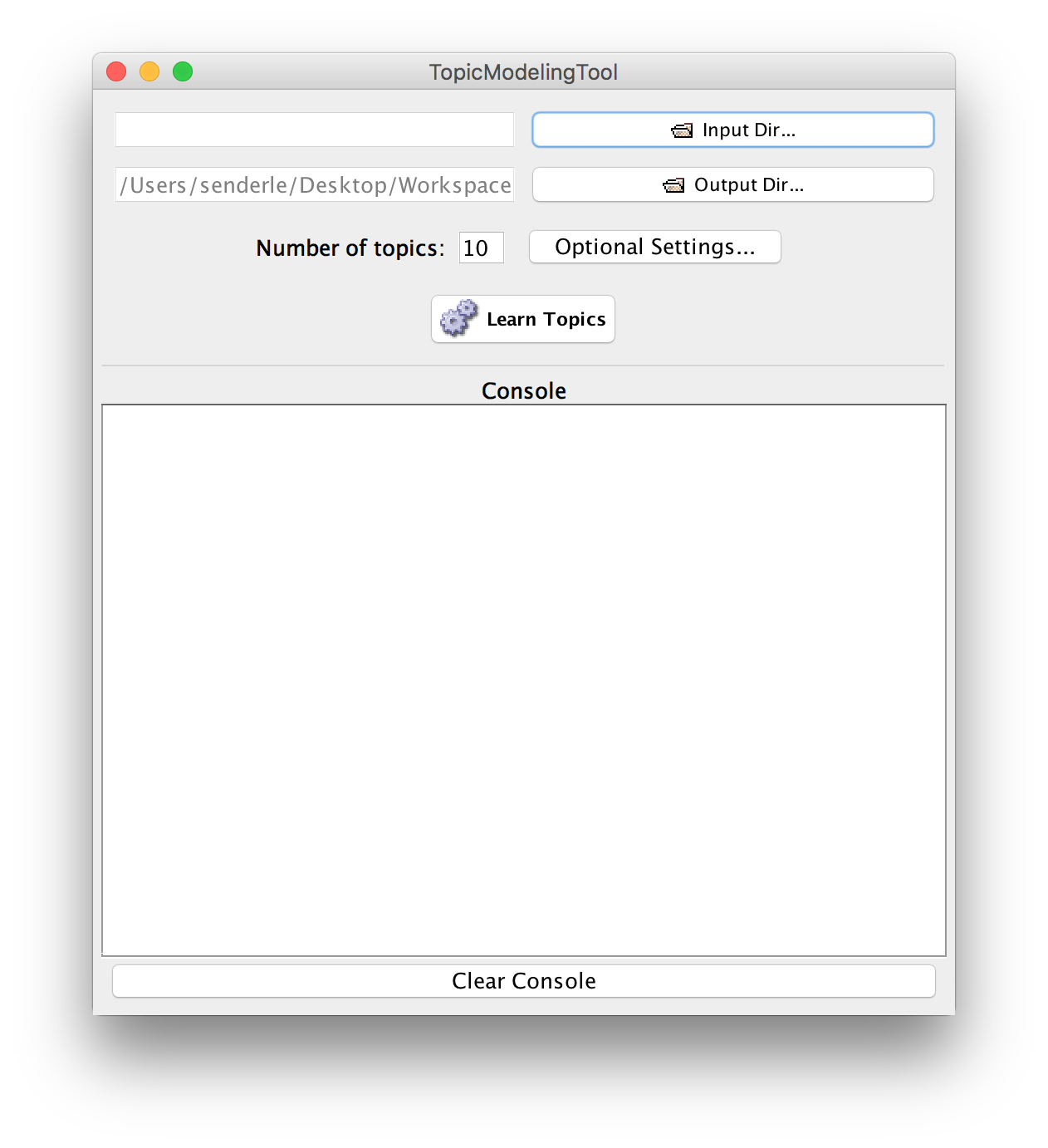
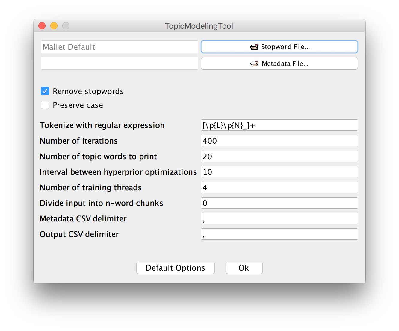
- what other options are present under 'advanced'? What do you think they do?
- Let's begin by exploring for 10 topics

(more info on the [optional settings here](https://senderle.github.io/topic-modeling-tool/documentation/2018/09/27/optional-settings.html0))

---

- Once the model has run, take a look at the 'output_html' folder using your browser (click on the 'index.html' file in there).
- look at the topics. Do they seem to capture _too many_ ideas? Too few? Try experimenting with more topics. Write your results to a different folder so that you can compare.
- Do you notice words or other things that seem to be not useful? See if you can figure out how to add these to the stopwords.
- Which number captures the seeming diversity of discourses here?

---

- following Senderle's [_quickstart_](https://senderle.github.io/topic-modeling-tool/documentation/2017/01/06/quickstart.html) try to visualize your results using Excel and pivot tables.
- what can you say about these materials, not having read them? _distant reading ftw!_

---

# Visualizing the ways documents inter-relate with a network

- a network visualization helps us explore the web of interconnected relationships in a body of material
- just because something _can_ be represented as a network doesn't mean it _should_
- We'll use [gephi](http://gephi.org)

---

## getting data into shape

- Look at the output_csv file.
- look at the topics-in-docs.csv file

it'll look a bit like this:

filename | toptopics | ... |...|...|
|---|---|---|---|---|
file:/Users/shawngraham/Documents/nls-text-chapbooks/104186076.txt | 2 | 0.61007239 | 1 | 0.340982387 |

---

- after the filename, you get the topic and how much it contributes to the composition of that document
- and then the next topic, its %, then the next topic.

- When we turn this into a network, it is going to be a _weighted_ network, where each relationship has a 'strength' value that corresponds to that percentage

- it's also going to be a _two mode_ network, because each 'node' in the network (in our case, each document) will be connected to a different kind of _thing_ - a topic

- two-mode networks hold value in terms of their _visual rhetoric_ but **nb** nearly all network statistics assume one-mode networks.

---

- let's make a network file from the topics-in-docs.csv file
- copy the list of filenames into a new spreadsheet.
- use 'find' to find the filepath from the filename, and 'replace' the path with a space so that you are left with just the filename
- eg: file:/Users/shawngraham/Documents/nls-text-chapbooks/104186076.txt
- find: "file:/Users/shawngraham/Documents/nls-text-chapbooks/"
- replace: ""
- result: "104186076.txt"
- (you can do the same thing again to get rid of .txt)

---

- copy the first column of topics, and paste appropriately in your new spreadsheet
- copy the first column of percentages and paste appropriately
- insert at the top of your data 'source','target','weight' for column names

- copy the document names again, and insert at the bottom of your new sheet
- copy the next column of topics and percentages appropriately

- Save this file as 'topicnetwork.csv'
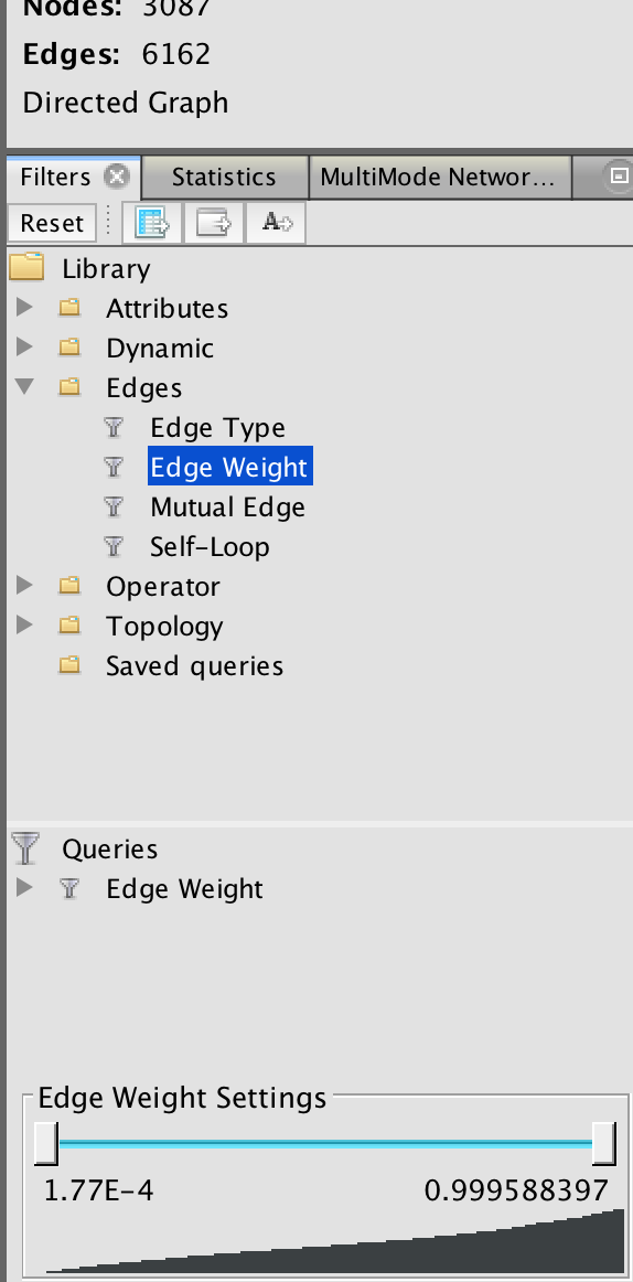
- **warning** you might want to consider now filtering this list so only the top third of strong relationships are present.

---

## load that into gephi

- open Gephi
- open graph file
- select topicnetwork.csv
- in dialogue, make sure it says 'edges' table



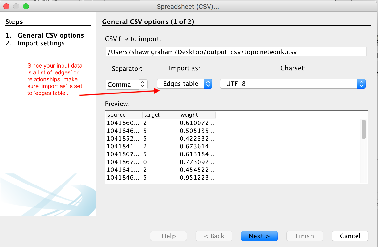
- click finish

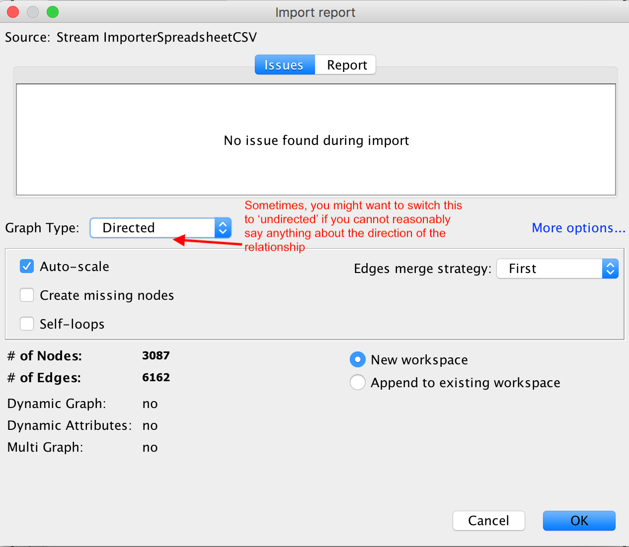
It will import your network, present you with a report on the results of the import. Click ok.

---

A mass of nodes/edges appears.
- under 'layout' on the bottom left panel, click 'force atlas 2' and then run. Hit the stop button after a few moments.



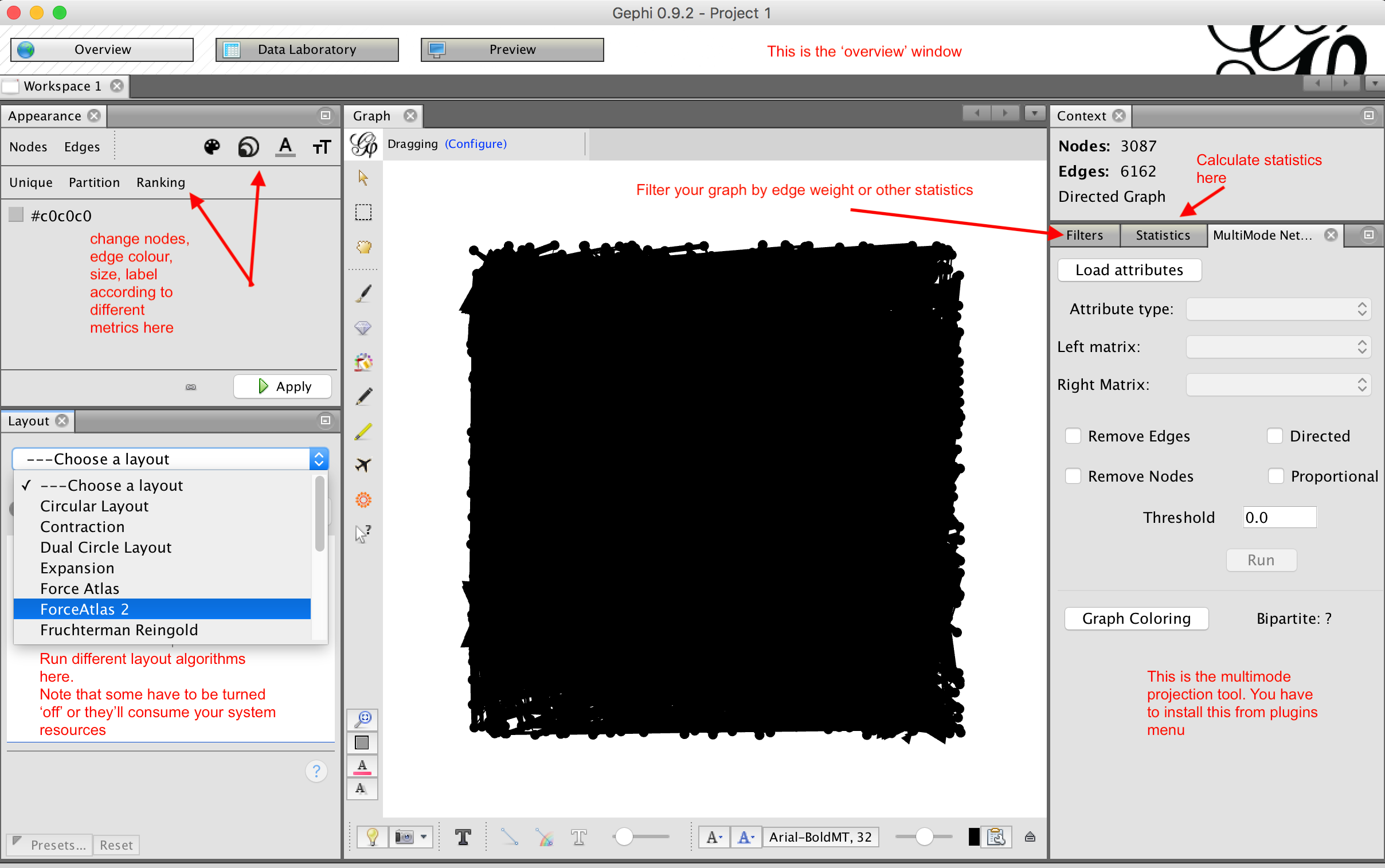
play with the interface for a bit.

---

## Convert from two mode to one mode

To convert from two mode to one mode:

- tools > plugins > available plugins
- select 'MultimodeNetworkTransformation'


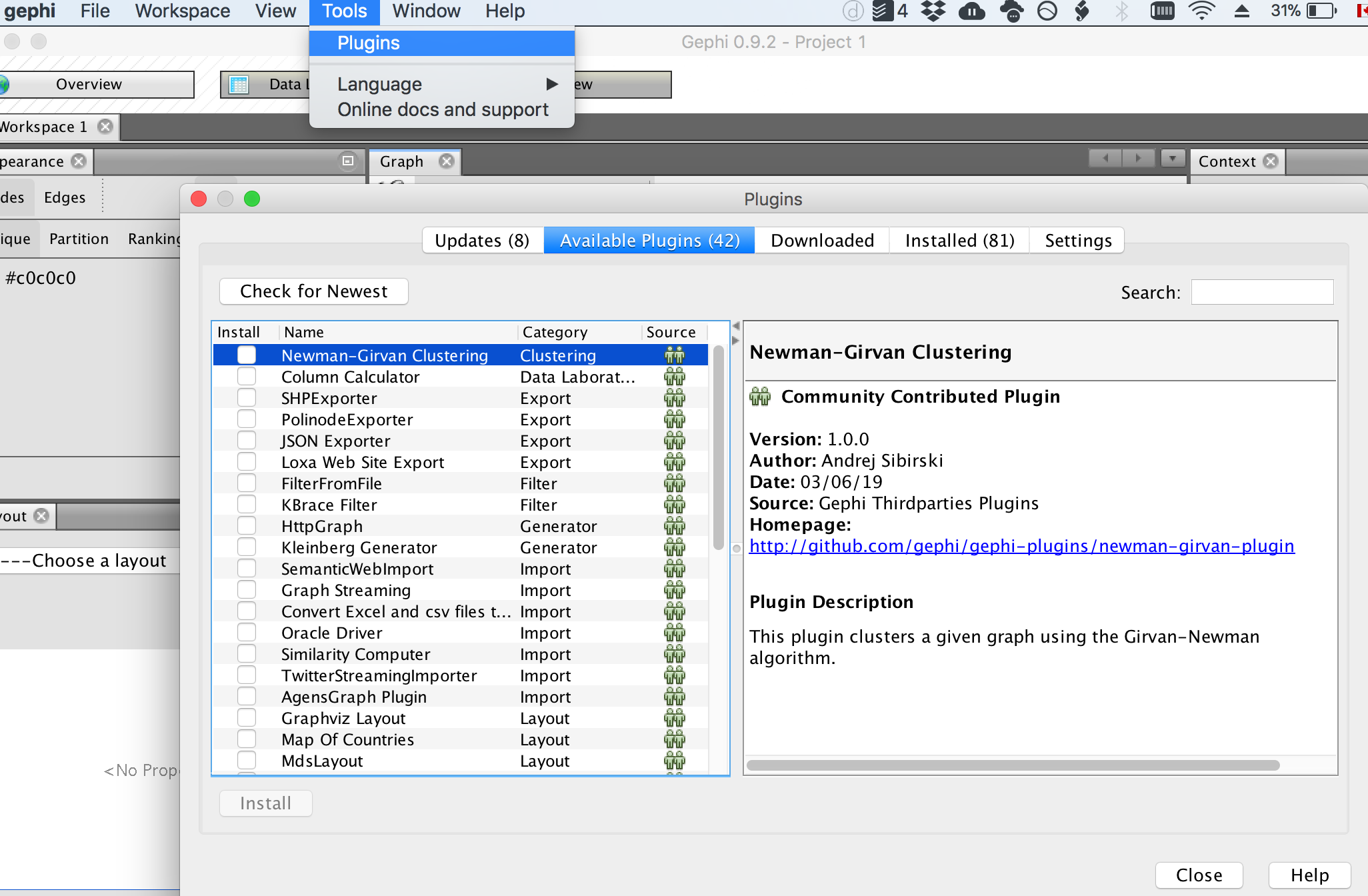
- install it. You'll probably have to restart Gephi. Don't save your work

---

- Restart gephi.
- open your network file
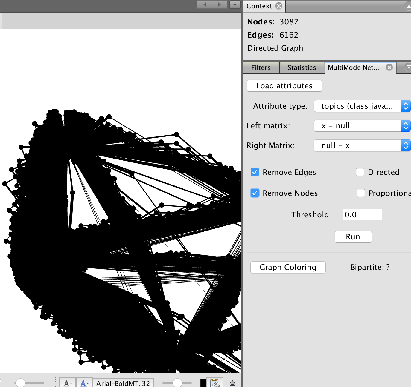
- the multimode network tool is now in a panel on the right-hand side of your workspace


---

We have to tell Gephi which rows of data correspond with our topics.

- click on 'data laboratory'
- click on 'nodes'
- click on 'add column'
- call it 'Topic'


---

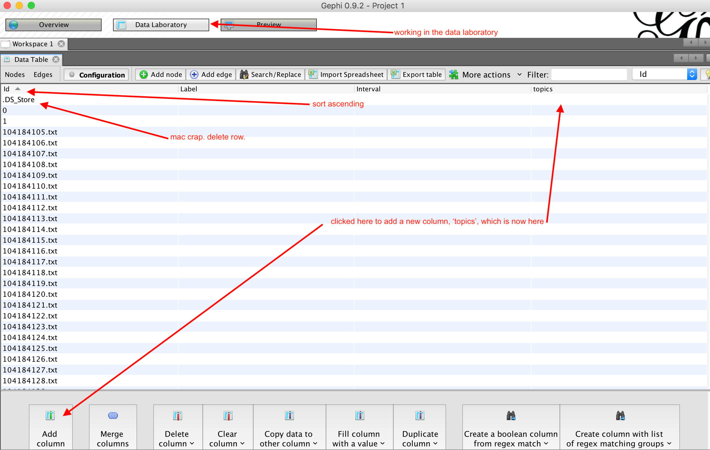
- Sort the nodes by clicking on 'id' column
- in each row of your data where there is a topic, click on the relevant cell in 'Topic' column and add an X


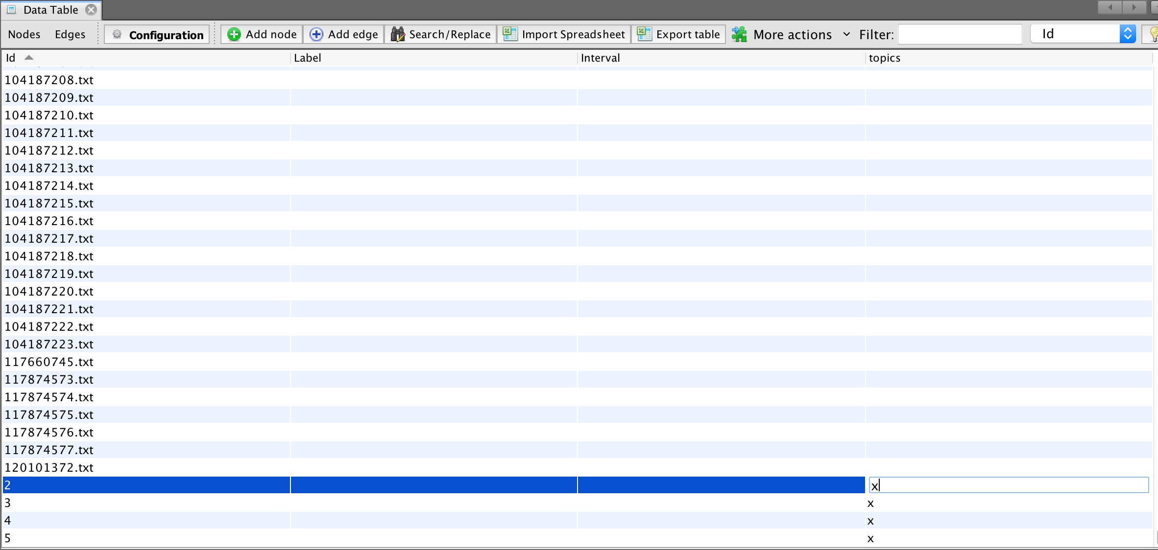
- save your work

---

- click on overview window
- in the multimode network tool, choose 'load attributes'
- What we are about to do now will change your data.
- in 'attribute type' select 'topic'
- in the left matrix, select 'null-x'

_this is going to make a document to document network by virtue of shared topic; to create the opposite you'd select x-null'_

---

- if you are doing document - document by virtue of shared topics, consider placing a threshold value of 0.75 - ie, only reproject those relationships at 0.75 or stronger.
- select 'remove nodes'
- select 'remove edges'
- click on 'run'


---

Save your work under a new name, like 'network-docs-to-docs'

To project your data the opposite way, reload your original data and reverse.

---

## Some stats

Now we can run some stats. Useful here is probably 'modularity' which will find 'communities' of similar documents.

- stats are available on the right hand side of the 'overview' window
- you can alter the appearance of the network to reflect statistics for the edges and nodes in the 'appearance' panel on the left hand side
- conventions: colour by modularity, resize by centrality

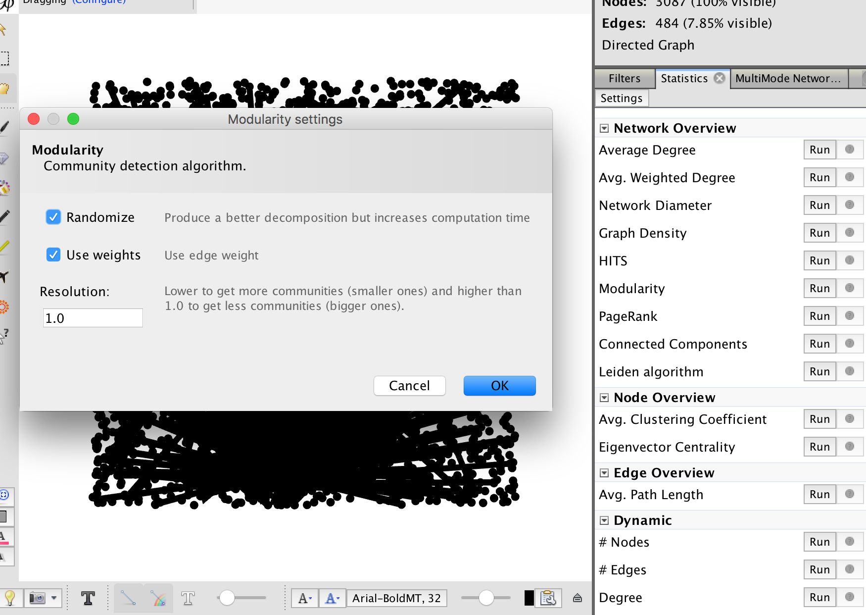
Selecting stats, then modularity to find 'communities' of nodes with similar patterns of linkages.

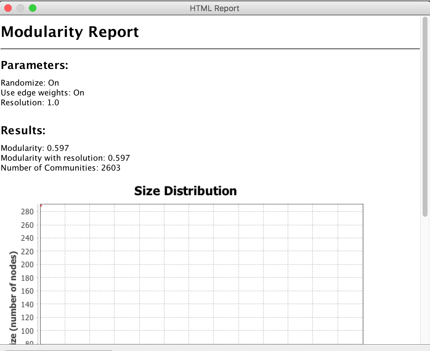
Every statistical test will give you a report and visualization of the results. With regard to modularity, you want to get a score as close to 1 as possible. The closer to 1, the more likely the results are 'real'.

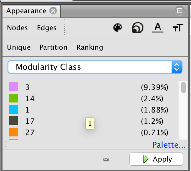
After you run a stat, you can update the display to take this new information into account. It is also made available as a new column in your data table (either for nodes or edges as appropriate). Here, we clicked 'nodes' then 'partition' and selected from the values that then appeared eg modularity. Once we hit apply, the nodes will colour according to whichever module they are a part of.

---

## Export as a website

- save your work

- under plugins you can find a web export tool called 'sigma exporter'
- find that, install it, give it a spin
- select where you want to save the resulting website
- fill in the fields as appropriate

----

## View in browser

If you're on a mac, open a new terminal where you saved it, then at the prompt start a server with `python -m SimpleHTTPServer`

In your browser, go to `localhost:8000` and you'll see your visualization!

- all of these files can be loaded into a github repository and served on the web.