# Lecture 2: Classification and CNNs
## Introduction
In this section we will introduce the Image Classification problem, which is the task of assigning an input image one label from a fixed set of categories. This is one of the core problems in Computer Vision that, despite its simplicity, has a large variety of practical applications.

>[[1]](#cs231n) Reference: https://cs231n.github.io/classification/

### Motivation (why CNNs?)
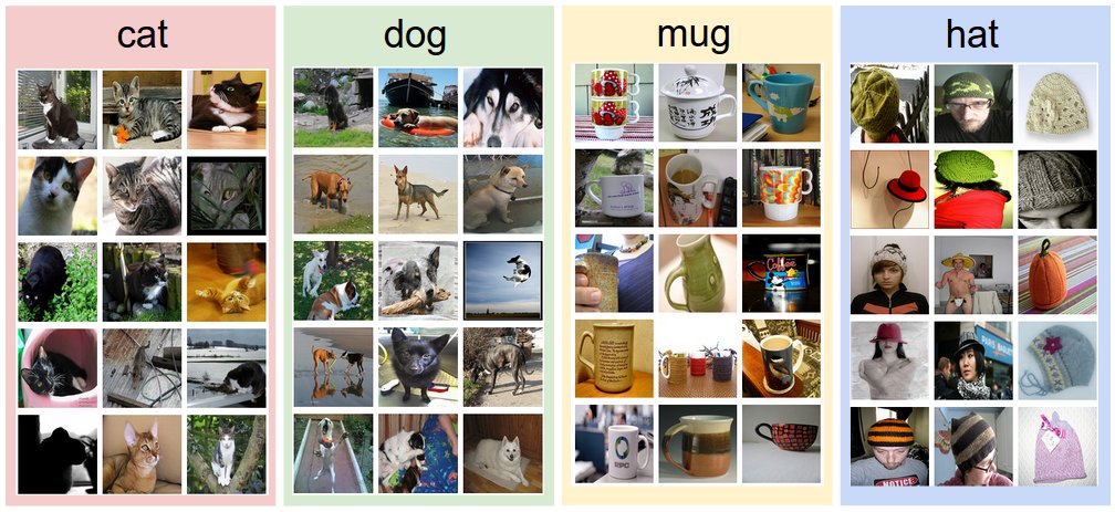
An example of image classification: looking at an image of a pet and deciding whether it’s a cat or a dog. A common solution to this task is Convolutional Neural Networks (CNNs).
**Question:** why not just use a normal Feedforward Neural Network (FFN)?
- **Images are big (have large resolutions).** Images used for Computer Vision problems nowadays are often 224 x 224 or larger. Imagine building a neural network to process 224 x 224 color images: including the 3 color channels (RGB) in the image, which comes out to 224 x 224 x 3 = 150,528 input features! A typical hidden layer in such a network might have 1024 nodes, so we’d have to train 150,528 x 1024 = 150+ million weights for the first layer alone. Our network would be huge and nearly impossible to train. It’s not like we need that many weights, either.
- **Images contain rich spatial information.** The nice thing about images is that we know pixels are most useful in the context of their neighbors. Objects in images are made up of small, localized features, like the circular iris of an eye or the square corner of a piece of paper. Therefore, convolution on two or more dimensional data is more suitable for image classification.
- **Positions can change.** If you trained a network to detect dogs, you’d want it to be able to detect a dog regardless of where it appears in the image. Imagine training a network that works well on a certain dog image, but then feeding it a slightly shifted version of the same image. The dog would not activate the same neurons, so the network would react completely differently!

## CNN Basis
There are several types of layers typically used to construct CNN:
- convolution layer
- pooling layer
- batch normlization layer
- activation layer


Here we first describe the numerical representation of images and then detail each abovementioned layer.

### Numerical representation of images
An image on a computer screen is made up of pixels (dots). Each of these pixels, is merely a brightness level. For a gray scale (black-and-white or monochrome) image these typically range from $0$ for no brightness (black) to $255$ for full brightness (white).

A gray scale image can therefor be represented as a rank-2 tensor (a matrix), with row and column numbers equal to the dimensions of height and width of the image.

A $5 \times 5$ gray scale image that is totally black is shown as a matrix in (1) below.

$$ \begin{bmatrix} 0 & 0 & 0 & 0 & 0 \\ 0 & 0 & 0 & 0 & 0 \\ 0 & 0 & 0 & 0 & 0 \\ 0 & 0 & 0 & 0 & 0 \\ 0 & 0 & 0 & 0 & 0 \end{bmatrix} \tag{1} $$

Color images are made up of three such brightness value layers, one each for red, green, and blue. This is represented numerically by a rank-3 tensor. The three layers are referred to as _channels_. The same black image above, when viewed as a color image, would have dimension of $5 \times 5 \times 3$.

### The convolution layer
The convolution operation forms the basis of a CNN. Consider the two $3 \times 3$ matrices in (2) below.

$$ \begin{bmatrix} 1 & 2 & 3 \\ 4 & 3 & 3 \\ 3 & 4 & 2 \end{bmatrix} \begin{bmatrix} 3 & 3 & 2 \\ 1 & 1 & 2 \\ 7 & 2 & 2 \end{bmatrix} \tag{2}$$

The convolutional operation multiplies the corresponding values (by index or address) and adds all these products. The result is shown in (3) below.

$$\left(1 \times 3\right) + \left(2 \times 3\right) + \left(3 \times 2\right) + \\ \left(4 \times 1\right) + \left(3 \times 1\right) + \left(3 \times 2\right) + \\ \left(3 \times 7\right) + \left(4 \times 2\right) + \left(2 \times 2\right) \\ = 3 + 6 + 6 +4 +3+6+21+8+4 \\ = 61\tag{3}$$

There is more to the convolution operation, though. Images are usually larger than $3$ pixels wide and high. Consider then a very small, square image that is $10$ pixels on either side. The first $3 \times 3$ matrix in the example above is placed in the upper left corner of the image, so that a $3 \times 3$ area overlaps. A similar multiplication and addition operation ensues, resulting in a scalar value. This becomes the top-left pixel in the resultant _image_. In this course the _resultant image_ will refer to the data for the next layer. The $3 \times 3$ matrix now moves on one pixel to the tight of the image and the calculation is repeated, resulting in the second pixel value of the resultant image. When the $3 \times 3$ matrix runs up against the right edge of the image and performs the same calculation, it then moves one pixel down and jumps all the way to the left. This process continues until the $3 \times 3$ matrix ends up at the bottom right of the image. This is the convolution operation and is depicted below.

> [[2]](#conv12) Reference: https://towardsdatascience.com/a-comprehensive-introduction-to-different-types-of-convolutions-in-deep-learning-669281e58215

**Kernel Size.** Kernel size can be 5 x 5, 3 x 3, and so on. Larger filter sizes should be avoided as the learning algorithm needs to learn filter values (weights), and larger filters increase the number of weights to be learned (more compute capacity, more training time, more chance of overfitting). Also, odd sized filters are preferred to even sized filters, due to the nice geometric property of all the input pixels being around the output pixel.

**Padding.** It follows from the description of the convolution operation above that pixels away from the edge are _more involved_ in the learning process. To aid in the edge pixels contributing to the process and to prevent the resultant image from being smaller, _padding_ can be employed to the original image. If padding=1, an edge of zero values are added all around the image. Where it was $n \times n$ before, it becomes $\left( n + 2 \right) \times \left( n + 2 \right)$ in size. Note that this is the specific case of a kernel with and odd size, i.e. $3 \times 3$.

**Stride.** The process described so far, has the kernel moving along and down, one pixel at a time. This is the _stride length_. A higher value for the stride length can be set. A stride length of two is shown below.

**Sample code.** 3x3 convolution in pytorch.

def conv3x3(in_channels, out_channels, stride=1):
    return nn.Conv2d(in_channels, out_channels, kernel_size=3, 
                     stride=stride, padding=1, bias=False)

### The Pooling layer
Pooling consolidates the resultant image by looking at square sized pixel grids, i.e. $2 \times 2$. This grid moves along the image as with the convolution operation. Max pooling is most commonly used. In the grid formed by a $2 \times 2$ square pixel area, the largest value is maintained in a new resultant image.

**Average pooling**, where the average of the values in the grid is calculated, can also be used. It has not been shown to be of much benefit and was used prior to the current era of deep learning.

**Max pooling** for a $2 \times 2$ grid is shown below. The maximum value in the first grid is $78$, which is the maximum value in the first pixel of the resultant image. It remains the maximum value as the grid moves one pixel to the right, and so on.

### The Batch Normlization layer
Data normalization (or feature scaling) is important in CNNs for stable training. One can normalize the output of hidden layer to increase stability of a network. Normalization (usually) helps to train the network.

The idea of batch normalization is to make activations unit gaussian by scaling the input $x$.

Let $X = \{x_1, \cdots, x_N\}$ be a batch of $D$-dimensional vectors. We define *mini-batch mean* and *mini-batch variance*:

\begin{eqnarray}
\mu & = & \frac{1}{N}\sum\limits_{i=1}^{N}x_i \\
\sigma^2 & = & \frac{1}{N}\sum\limits_{i=1}^{N}\left(x_i - \mu\right)^2
\end{eqnarray}

Note, that $\mu, \sigma^2 \in\mathcal{R}^D$, and normalized input: $\hat x_i = \frac{x_i - \mu}{\sqrt{\sigma^2 + \varepsilon}}$, where $\varepsilon << 1$ is just to ensure denominator not equal zero.

Please note, that in the original paper the mean and the variance are calculated for batch (during training) and for the whole training dataset (during inference).

### The Activation layer
Simply put, an activation function is a function that is added into an artificial neural network in order to help the network learn complex patterns in the data. Every activation function (or non-linearity) takes a single number and performs a certain fixed mathematical operation on it. There are several activation functions you may encounter in practice.

**Sigmoid:** The sigmoid is defined as:
This activation function is here only for historical reasons and never used in real models. It is computationally expensive, causes vanishing gradient problem and not zero-centred. This method is generally used for binary classification problems.

**Softmax:** The softmax is a more generalised form of the sigmoid. It is used in multi-class classification problems. Similar to sigmoid, it produces values in the range of 0–1 therefore it is used as the final layer in classification models.

**Tanh:** The tanh is defined as:
If you compare it to sigmoid, it solves just one problem of being zero-centred.

**ReLU:**: ReLU (Rectified Linear Unit) is defined as f(x) = max(0,x):
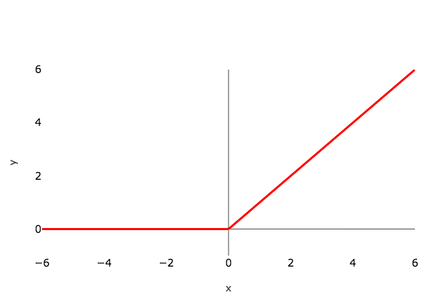
This is a widely used activation function, especially with Convolutional Neural networks. It is easy to compute and does not saturate and does not cause the Vanishing Gradient Problem. It has just one issue of not being zero centred.

### The Flattening operation
Before an output layer can be constructed, the last resultant image must be flattened, i.e. turned into a vector. Each pixel is simply taken from top-left, moving along the current row, before dropping down one row and restarting at the left until to bottom-right is reached. This is then passed through a densely connected layer.

## CNN Architectures
As we described above, a simple ConvNet is a sequence of layers, and every layer of a ConvNet transforms one volume of activations to another through a differentiable function. We use three main types of layers to build ConvNet architectures: **Convolutional Layer, Pooling Layer, Normlization Layer, Activation Layer, and Fully-Connected Layer** (exactly as seen in regular Neural Networks). We will stack layers to form a full ConvNet architecture.

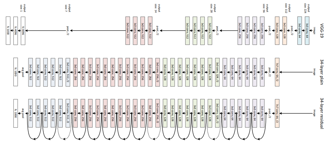
### VGG

This architecture is from VGG group, Oxford. It makes the improvement over AlexNet by replacing large kernel-sized filters(11 and 5 in the first and second convolutional layer, respectively) with multiple 3 x 3 kernel-sized filters one after another. With a given receptive field(the effective area size of input image on which output depends), multiple stacked smaller size kernel is better than the one with a larger size kernel because multiple non-linear layers increases the depth of the network which enables it to learn more complex features, and that too at a lower cost.

For example, three 3 x 3 filters on top of each other with stride 1 ha a receptive size of 7, but the number of parameters involved is $3*(9C^2)$ in comparison to $49C^2$ parameters of kernels with a size of 7. Here, it is assumed that the number of input and output channel of layers is $C$. Also, 3 x 3 kernels help in retaining finer level properties of the image. The network architecture is given in the table.

**Sample code.** VGGNet in Pytorch.

import torch
import torch.nn as nn
from typing import Union, List, Dict, Any, cast

class VGG(nn.Module):

    def __init__(
        self,
        features: nn.Module,
        num_classes: int = 1000,
        init_weights: bool = True
    ) -> None:
        super(VGG, self).__init__()
        self.features = features
        self.avgpool = nn.AdaptiveAvgPool2d((7, 7))
        self.classifier = nn.Sequential(
            nn.Linear(512 * 7 * 7, 4096),
            nn.ReLU(True),
            nn.Dropout(),
            nn.Linear(4096, 4096),
            nn.ReLU(True),
            nn.Dropout(),
            nn.Linear(4096, num_classes),
        )
        if init_weights:
            self._initialize_weights()

    def forward(self, x: torch.Tensor) -> torch.Tensor:
        x = self.features(x)
        x = self.avgpool(x)
        x = torch.flatten(x, 1)
        x = self.classifier(x)
        return x

    def _initialize_weights(self) -> None:
        for m in self.modules():
            if isinstance(m, nn.Conv2d):
                nn.init.kaiming_normal_(m.weight, mode='fan_out', nonlinearity='relu')
                if m.bias is not None:
                    nn.init.constant_(m.bias, 0)
            elif isinstance(m, nn.BatchNorm2d):
                nn.init.constant_(m.weight, 1)
                nn.init.constant_(m.bias, 0)
            elif isinstance(m, nn.Linear):
                nn.init.normal_(m.weight, 0, 0.01)
                nn.init.constant_(m.bias, 0)


def make_layers(cfg: List[Union[str, int]], batch_norm: bool = False) -> nn.Sequential:
    layers: List[nn.Module] = []
    in_channels = 3
    for v in cfg:
        if v == 'M':
            layers += [nn.MaxPool2d(kernel_size=2, stride=2)]
        else:
            v = cast(int, v)
            conv2d = nn.Conv2d(in_channels, v, kernel_size=3, padding=1)
            if batch_norm:
                layers += [conv2d, nn.BatchNorm2d(v), nn.ReLU(inplace=True)]
            else:
                layers += [conv2d, nn.ReLU(inplace=True)]
            in_channels = v
    return nn.Sequential(*layers)


cfgs: Dict[str, List[Union[str, int]]] = {
    'A': [64, 'M', 128, 'M', 256, 256, 'M', 512, 512, 'M', 512, 512, 'M'],
    'B': [64, 64, 'M', 128, 128, 'M', 256, 256, 'M', 512, 512, 'M', 512, 512, 'M'],
    'D': [64, 64, 'M', 128, 128, 'M', 256, 256, 256, 'M', 512, 512, 512, 'M', 512, 512, 512, 'M'],
    'E': [64, 64, 'M', 128, 128, 'M', 256, 256, 256, 256, 'M', 512, 512, 512, 512, 'M', 512, 512, 512, 512, 'M'],
}


def _vgg(arch: str, cfg: str, batch_norm: bool, pretrained: bool, progress: bool, **kwargs: Any) -> VGG:
    if pretrained:
        kwargs['init_weights'] = False
    model = VGG(make_layers(cfgs[cfg], batch_norm=batch_norm), **kwargs)
    if pretrained:
        state_dict = load_state_dict_from_url(model_urls[arch],
                                              progress=progress)
        model.load_state_dict(state_dict)
    return model

### ResNet
Neural Networks are notorious for not being able to find a simpler mapping when it exists.
- For example, say we have a fully connected multi-layer perceptron network and we want to train it on a data-set where the input equals the output. The simplest solution to this problem is having all weights equaling one and all biases zeros for all the hidden layers. But when such a network is trained using back-propagation, a rather complex mapping is learned where the weights and biases have a wide range of values.
- Another example is adding more layers to an existing neural network. Say we have a network f(x) that has achieved an accuracy of n% on a data-set. Now adding more layers to this network g(f(x)) should have at least an accuracy of n% i.e. in the worst case g(.) should be an identical mapping yielding the same accuracy as that of f(x) if not more. But unfortunately, that is not the case. Experiments have shown that the accuracy decreases by adding more layers to the network.
- The issues mentioned above happens because of the vanishing gradient problem. As we make the CNN deeper, the derivative when back-propagating to the initial layers becomes almost insignificant in value.

**ResNet** addresses this network by introducing two types of **shortcut connections**: Identity shortcut and Projection shortcut.
There are multiple versions of ResNetXX architectures where ‘XX’ denotes the number of layers. The most commonly used ones are ResNet18, ResNet34, ResNet50 and ResNet101. Since the vanishing gradient problem was taken care of, CNN started to get deeper and deeper. Below we present the structural details of ResNet18.

Resnet18 has around 11 million trainable parameters. It consists of CONV layers with filters of size 3x3 (just like VGGNet). Only two pooling layers are used throughout the network one at the beginning and the other at the end of the network. Identity connections are between every two CONV layers. The solid arrows show identity shortcuts where the dimension of the input and output is the same, while the dotted ones present the projection connections where the dimensions differ.

As mentioned earlier, ResNet architecture makes use of shortcut connections to solve the vanishing gradient problem. The basic building block of ResNet is a Residual block that is repeated throughout the network.

Instead of learning the mapping from x -> F(x), the network learns the mapping from x -> F(x)+G(x). When the dimension of the input x and output F(x) is the same, the function G(x) = x is an identity function and the shortcut connection is called Identity connection. The identical mapping is learned by zeroing out the weights in the intermediate layer during training since it's easier to zero out the weights than push them to one.

For the case when the dimensions of F(x) differ from x (due to stride length > 1 in the CONV layers in between), the Projection connection is implemented rather than the Identity connection. The function G(x) changes the dimensions of input x to that of output F(x). Two kinds of mapping were considered in the original paper.


**Sample code.** A basic block of ResNet.

class BasicBlock(nn.Module):
    expansion = 1

    def __init__(self, inplanes, planes, stride=1, downsample=None, groups=1,
                 base_width=64, dilation=1, norm_layer=None):
        super(BasicBlock, self).__init__()
        if norm_layer is None:
            norm_layer = nn.BatchNorm2d
        if groups != 1 or base_width != 64:
            raise ValueError('BasicBlock only supports groups=1 and base_width=64')
        if dilation > 1:
            raise NotImplementedError("Dilation > 1 not supported in BasicBlock")
        # Both self.conv1 and self.downsample layers downsample the input when stride != 1
        self.conv1 = conv3x3(inplanes, planes, stride)
        self.bn1 = norm_layer(planes)
        self.relu = nn.ReLU(inplace=True)
        self.conv2 = conv3x3(planes, planes)
        self.bn2 = norm_layer(planes)
        self.downsample = downsample
        self.stride = stride

    def forward(self, x):
        identity = x

        out = self.conv1(x)
        out = self.bn1(out)
        out = self.relu(out)

        out = self.conv2(out)
        out = self.bn2(out)

        if self.downsample is not None:
            identity = self.downsample(x)

        out += identity
        out = self.relu(out)

        return out

## Convolution Variants [[Reference](https://towardsdatascience.com/a-comprehensive-introduction-to-different-types-of-convolutions-in-deep-learning-669281e58215)]
### Dilated Convolution (Atrous Convolution)
Dilated convolution was introduced in the paper "Multi-scale context aggregation by dilated convolutions". Intuitively, dilated convolutions “inflate” the kernel by inserting spaces between the kernel elements. This additional parameter l (dilation rate) indicates how much we want to widen the kernel. Implementations may vary, but there are usually l-1 spaces inserted between kernel elements. The following image shows the kernel size when l = 1, 2, and 4.

> Reference: https://towardsdatascience.com/a-comprehensive-introduction-to-different-types-of-convolutions-in-deep-learning-669281e58215

In the image, the 3 x 3 red dots indicate that after the convolution, the output image is with 3 x 3 pixels. Although all three dilated convolutions provide the output with the same dimension, the receptive field observed by the model is dramatically different. The receptive filed is 3 x 3 for l =1. It is 7 x 7 for l =2. The receptive filed increases to 15 x 15 for l = 3. Interestingly, the numbers of parameters associated with these operations are essentially identical. We “observe” a large receptive filed without adding additional costs. Because of that, dilated convolution is used to cheaply increase the receptive field of output units without increasing the kernel size, which is especially effective when multiple dilated convolutions are stacked one after another.

The authors in the paper “Multi-scale context aggregation by dilated convolutions” build a network out of multiple layers of dilated convolutions, where the dilation rate l increases exponentially at each layer. As a result, the effective receptive field grows exponentially while the number of parameters grows only linearly with layers! Please check out the paper for more information.

**Code:**
> torch.nn.Conv2d(in_channels, out_channels, kernel_size, stride=1, padding=0, **dilation**=1, groups=1, bias=True, padding_mode='zeros', device=None, dtype=None)

### Depthwise Convolutions
Let’s have a quick recap of standard 2D convolutions. For a concrete example, let’s say the input layer is of size 7 x 7 x 3 (height x width x channels), and the filter is of size 3 x 3 x 3. After the 2D convolution with one filter, the output layer is of size 5 x 5 x 1 (with only 1 channel).


Typically, multiple filters are applied between two neural net layers. Let’s say we have 128 filters here. After applying these 128 2D convolutions, we have 128 5 x 5 x 1 output maps. We then stack these maps into a single layer of size 5 x 5 x 128. By doing that, we transform the input layer (7 x 7 x 3) into the output layer (5 x 5 x 128). The spatial dimensions, i.e. height & width, are shrunk, while the depth is extended.


Now we apply depthwise convolution to the input layer. Instead of using a single filter of size 3 x 3 x 3 in 2D convolution, we used 3 kernels, separately. Each filter has size 3 x 3 x 1. Each kernel convolves with 1 channel of the input layer (1 channel only, not all channels!). Each of such convolution provides a map of size 5 x 5 x 1. We then stack these maps together to create a 5 x 5 x 3 image. After this, we have the output with size 5 x 5 x 3. We now shrink the spatial dimensions, but the depth is still the same as before.


**Code:**
> torch.nn.Conv2d(in_channels, out_channels, kernel_size, stride=1, padding=0, dilation=1, **groups=in_channels**, bias=True, padding_mode='zeros', device=None, dtype=None)

### Grouped Convolution
Here we describe how the grouped convolutions work. First of all, conventional 2D convolutions follow the steps showing below. In this example, the input layer of size (7 x 7 x 3) is transformed into the output layer of size (5 x 5 x 128) by applying 128 filters (each filter is of size 3 x 3 x 3). Or in general case, the input layer of size (Hin x Win x Din) is transformed into the output layer of size (Hout x Wout x Dout) by applying Dout kernels (each is of size h x w x Din).

In grouped convolution, the filters are separated into different groups. Each group is responsible for a conventional 2D convolutions with certain depth. The following examples can make this clearer.


Above is the illustration of grouped convolution with 2 filter groups. In each filter group, the depth of each filter is only half of the that in the nominal 2D convolutions. They are of depth Din / 2. Each filter group contains Dout /2 filters. The first filter group (red) convolves with the first half of the input layer ([:, :, 0:Din/2]), while the second filter group (blue) convolves with the second half of the input layer ([:, :, Din/2:Din]). As a result, each filter group creates Dout/2 channels. Overall, two groups create 2 x Dout/2 = Dout channels. We then stack these channels in the output layer with Dout channels.

**Code:**
> torch.nn.Conv2d(in_channels, out_channels, kernel_size, stride=1, padding=0, dilation=1, **groups=2**, bias=True, padding_mode='zeros', device=None, dtype=None)

### Shuffled Grouped Convolution
Overall, the shuffled grouped convolution involves grouped convolution and channel shuffling. In the section about grouped convolution, we know that the filters are separated into different groups. Each group is responsible for a conventional 2D convolutions with certain depth. The total operations are significantly reduced. For examples in the figure below, we have 3 filter groups. The first filter group convolves with the red portion in the input layer. Similarly, the second and the third filter group convolves with the green and blue portions in the input. The kernel depth in each filter group is only 1/3 of the total channel count in the input layer. In this example, after the first grouped convolution GConv1, the input layer is mapped to the intermediate feature map. This feature map is then mapped to the output layer through the second grouped convolution GConv2.

Grouped convolution is computationally efficient. But the problem is that each filter group only handles information passed down from the fixed portion in the previous layers. For examples in the image above, the first filter group (red) only process information that is passed down from the first 1/3 of the input channels. The blue filter group (blue) only process information that is passed down from the last 1/3 of the input channels. As such, each filter group is only limited to learn a few specific features. This property blocks information flow between channel groups and weakens representations during training. To overcome this problem, we apply the channel shuffle.

The idea of channel shuffle is that we want to mix up the information from different filter groups. In the image below, we get the feature map after applying the first grouped convolution GConv1 with 3 filter groups. Before feeding this feature map into the second grouped convolution, we first divide the channels in each group into several subgroups. The we mix up these subgroups.


After such shuffling, we continue performing the second grouped convolution GConv2 as usual. But now, since the information in the shuffled layer has already been mixed, we essentially feed each group in GConv2 with different subgroups in the feature map layer (or in the input layer). As a result, we allow the information flow between channels groups and strengthen the representations.

**Code for Channel Shuffle:**

def channel_shuffle(x: Tensor, groups: int) -> Tensor:
    batchsize, num_channels, height, width = x.size()
    channels_per_group = num_channels // groups

    # reshape
    x = x.view(batchsize, groups, channels_per_group, height, width)

    x = torch.transpose(x, 1, 2).contiguous()

    # flatten
    x = x.view(batchsize, -1, height, width)

    return x

class MyConv(nn.Module):
    def __init__(self):
        super(MyConv, self).__init__()
        
        self.g_conv1 = nn.Conv2d(32, 64, 3, 1, 1,groups=8)
        self.g_conv2 = nn.Conv2d(64, 64, 3, 1, 1,groups=8)
        self.conv3 = nn.Conv2d(64, 64, 1, 1)
        self.conv4 = nn.Conv2d(64, 64, 1, 1)

    def channel_shuffle(self, x, groups):
        
        batch_size, num_channels, height, width = x.size()
        channels_per_group = num_channels // groups
        x = x.view(batch_size, groups, channels_per_group, height, width)
        x = torch.transpose(x,1,2).contiguous()
        x = x.view(batch_size,-1,height,width)
        
        return x

        
    def forward(self, x):
 
        x = self.g_conv1(x)

        x = self.channel_shuffle(x,8)

        x = self.g_conv2(x)

        x = self.conv3(x)

        ## forward x to relu activation function.
        x = F.relu(x)
        
        x = self.conv4(x)
        return x
        

## Regularization of Neural Networks

### Why Regularization?
Overfitting is used to describe scenarios when the trained model doesn’t generalize well on unseen data but mimics the training data very well. As shown in the figure below, the **blue** line fits the training data extremely well, which always lead to bad performance on the test data. This fact is dubbed as "overfitting".

> Reference: https://www.machinecurve.com/wp-content/uploads/2020/01/poly_both.png

Adding regularization to your neural network, and specifically to the computed loss values, can help you in guiding the model towards learning a mapping that looks more like the one in **yellow**. Alternatively speaking, regularization avoids the model to be over-complicated that fit the training data extremely well.

### L1 Regularization
L1 regularization, also as known as Lasso regression, adds sum of the absolute values of all weights in the model to cost function. It shrinks the less important feature’s coefficient to zero thus, removing some features and hence providing a sparse solution.

Assuming that the task loss (e.g. cross entropy loss on classification task) is defined as $l_{task}$, and weight of $i$-th layer in the model is defined as $w_i$ , then we have the total loss as:

$l_{total} = l_{task} + \lambda \sum_i ||w_i||_1$, where $\lambda$ is a trade-off coefficient and $||\cdot ||_1$ means L1 norm.

**Sample code:**

# We need to define the task loss, e.g. cross entropy loss
# and define the model, e.g. ResNet

lambda = 0.01
l1_penalty = torch.nn.L1Loss(size_average=False)
reg_loss = torch.tensor(0.)
for param in model.parameters():
    reg_loss += l1_penalty(param)
loss += lambda * reg_loss

### L2 Regularization
L2 regularization, also as known as Ridge regression, adds sum of squares of all weights in the model to cost function. It is able to learn complex data patterns and gives non-sparse solutions unlike L1 regularization. The total loss that adds L2 regularization can be formulated as

$l_{total} = l_{task} + \lambda \sum_i ||w_i||_2$, where $\lambda$ is a trade-off coefficient and $||\cdot ||_2$ means L2 norm.

**Sample code:**

lambda = 0.01
reg_loss = torch.tensor(0.)
for param in model.parameters():
    reg_loss += torch.norm(param)
loss += lambda * reg_loss

### Difference between L1 and L2 Regularization
L1 regularization makes the weight sparse, i.e. lead some unimportant weights to zero, while L2 regualarization not. Let us analyse it from gradient. By using gradient descent to optimize parameter $w$ with objective $l(w)$, we have
\begin{eqnarray}
w = w - \alpha \frac{\partial l(w)}{\partial w}
\end{eqnarray}
where $\alpha$ is the learning rate. The gradient for L1 regularization part is:
\begin{eqnarray}
\frac{\partial ||w||_1}{\partial w} = sign(w)
\end{eqnarray}
The gradient for L2 regularization part is:
\begin{eqnarray}
\frac{\partial ||w||_2}{\partial w} = w
\end{eqnarray}
We can observe that the gradient for L1 regularization is $sign(w)$. It keeps +1 when $w$ is positive and -1 when $w$ is negative. The gradient for L2 regularization is $w$, which means the the gradient magnitude is correlated with weight magnitude itself. When $w$ has small magnitude, the graident for updating $w$ is small, therefore L1 regularization will lead to sparse weight, but not L2 regularization.

## FLOPs and Parameters
When doing deep learning on mobile devices, how good your model’s predictions are isn’t the only consideration. You also need to worry about:

- the amount of space the model takes up in your app bundle — a single model can add 100s of MBs to the download size of your app
- the amount of memory it takes up at runtime — on the iPhone and iPad the GPU can use all the RAM in the device, but that’s still only a few GB total, and when you run out of free memory the app gets terminated by the OS
- how fast the model runs — especially when working with live video or large images (if the model takes several seconds to process a single image you might be better off with a cloud service)
- how quickly it drains the battery — or makes the device too hot to hold!

### FLOPs
FLOPs (floating point of operations), is the number of floating point operations. It means the amount of calculation, which can be used to measure the algorithm / model complexity.

Many of the computations in neural networks are dot products, such as this:

`y = w[0]*x[0] + w[1]*x[1] + w[2]*x[2] + ... + w[n-1]*x[n-1]`

Here, w and x are two vectors, and the result y is a scalar (a single number). In the case of a convolutional layer or a fully-connected layer — the two main types of layers in modern neural networks — w would be the layer’s learned weights and x would be the input to that layer. y is one of the layer’s outputs. Typically a layer will have multiple outputs, and so we compute many of these dot products.

We count `w[0]*x[0] + ...` as one multiply-accumulate or 1 MACC. The “accumulation” operation here is addition, as we sum up the results of all the multiplications. The above formula has n of these MACCs.

Technically speaking there are only n - 1 additions in the above formula, one less than the number of multiplications. In terms of FLOPS, a dot product performs 2n - 1 FLOPS since there are n multiplications and n - 1 additions.

So a MACC is roughly two FLOPS, although multiply-accumulates are so common that a lot of hardware can do fused multiply-add operations where the MACC is a single instruction.

<!-- ### Parameters -->
Layers store their learned parameters, or weights, in main memory. In general, the fewer weights the model has, the small it is, and the faster it runs.

Now let’s look at a few different layer types to see how to compute the number of MACCs and Parameters for these layers.

**Fully-connected layer.** In a fully-connected layer, all the inputs are connected to all the outputs. For a layer with I input values and J output values, its weights W can be stored in an I × J matrix. The computation performed by a fully-connected layer is: `y = matmul(x, W) + b`.

Here, x is a vector of I input values, W is the I × J matrix containing the layer’s weights, and b is a vector of J bias values that get added as well. The result y contains the output values computed by the layer and is also a vector of size J.

To compute the number of MACCs, we look at where the dot products happen. For a fully-connected layer that is in the matrix multiplication `matmul(x, W)`.

A matrix multiply is simply a whole bunch of dot products. Each dot product is between the input x and one column in the matrix W. Both have I elements and therefore this counts as I MACCs. We have to compute J of these dot products, and so the total number of MACCs is I × J, the same size as the weight matrix.

The bias b doesn’t really affect the number of MACCs. Recall that a dot product has one less addition than multiplication anyway, so adding this bias value simply gets absorbed in that final multiply-accumulate.

Example: a fully-connected layer with 300 input neurons and 100 output neurons performs `300 × 100 = 30,000 MACCs`.

In general, multiplying a vector of length I with an I × J matrix to get a vector of length J, takes `I × J MACCs or (2I - 1) × J FLOPS`.

**Activation functions.** Usually a layer is followed by a non-linear activation function, such as a ReLU or a sigmoid. Naturally, it takes time to compute these activation functions. We don’t measure these in MACCs but in FLOPS, because they’re not dot products.

Some activation functions are more difficult to compute than others. For example, a ReLU is just:`y = max(x, 0)`.

This is a single operation on the GPU. The activation function is only applied to the output of the layer. On a fully-connected layer with J output neurons, the ReLU uses J of these computations, so let’s call this J FLOPS.

A sigmoid activation is more costly, since it involves taking an exponent: `y = 1 / (1 + exp(-x))`.

When calculating FLOPs we usually count addition, subtraction, multiplication, division, exponentiation, square root, etc as a single FLOP. Since there are four distinct operations in the sigmoid function, this would count as 4 FLOPs per output or J × 4 FLOPs for the total layer output.

**Convolutional layers.** The input and output to convolutional layers are not vectors but three-dimensional feature maps of size H × W × C where H is the height of the feature map, W the width, and C the number of channels at each location.

Most convolutional layers used today have square kernels. For a conv layer with kernel size K, the number of parameters of the convolutional layer is `K × K × Cin × Cout`. And the number of FLOPs is: `K × K × Cin × Hout × Wout × Cout`

For each pixel in the output feature map of size Hout × Wout, take a dot product of the weights and a K × K window of input values. We do this across all input channels, Cin
and because the layer has Cout different convolution kernels, we repeat this Cout times to create all the output channels. Note that we’re conveniently ignoring the bias and the activation function here.

Example: for a 3×3 convolution with 128 filters, on a 112×112 input feature map with 64 channels, we perform this many MACCs/FLOPs:
`3 × 3 × 64 × 112 × 112 × 128 = 924,844,032.`

**For group convolutions with a group number of $N_{group}$, the number of parameters of the convolutional layer is `K × K × Cin × Cout / Ngroup`, the number of FLOPs is: `K × K × Cin × Hout × Wout × Cout / Ngroup`.**

## References

<text id="cs231n"> [1]: https://cs231n.github.io/classification/
<text id="conv12"> [2]: https://towardsdatascience.com/a-comprehensive-introduction-to-different-types-of-convolutions-in-deep-learning-669281e58215
<text id="computation"> [3]: https://machinethink.net/blog/how-fast-is-my-model/
<text id="ReLU"> [4]: https://towardsdatascience.com/everything-you-need-to-know-about-activation-functions-in-deep-learning-models-84ba9f82c253
<text id="Pytorch"> [5]: https://pytorch.org/tutorials/