Virgil - EDA Visualization - S31 Time Series

--- title: Virgil - EDA Visualization - S31 Time Series tags: Virgil, LearnWorld, EDAVisualization --- <a target="_blank" href="https://colab.research.google.com/drive/1j2l_vlMEqsdU75rzMNjd1TgEMEWhQBFu"><img src="https://www.tensorflow.org/images/colab_logo_32px.png" />Run in Google Colab</a> # WORKING WITH TIME-SERIES <img src='https://media.giphy.com/media/jq07NJW0WA0I5Q7qQ4/giphy.gif' width=800> ## _Introduction_ **Pandas** was developed in the context of financial modeling, so as you might expect, it contains a fairly extensive set of tools for working with dates, times, and time-indexed data. Date and time data comes in a few flavors, which we will discuss here: ***Time stamps*** reference particular moments in time (e.g., July 4th, 2015 at 7:00am). 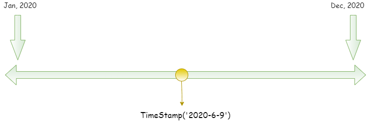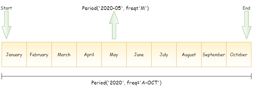![](https://miro.medium.com/max/1400/1*8uf_T4BqN0s5gbwWaPmXFg.png) ***Time intervals*** and ***periods*** reference a length of time between a particular beginning and end point; for example, the year 2015. Periods usually reference a special case of time intervals in which each interval is **of uniform length and does not overlap** (e.g., 24 hour-long periods comprising days). ![](https://miro.medium.com/max/1400/1*J1WOPRKuctCC_eAgQ-RwTw.png) ***Time deltas*** or ***durations*** reference an exact length of time (e.g., a duration of 22.56 seconds). In this section, we will introduce how to work with each of these types of date/time data in Pandas. This short section is by no means a complete guide to the time series tools available in Python or Pandas, but instead is intended as a broad overview of how you as a user should approach working with time series. We will start with a brief discussion of tools for dealing with dates and times in Python, before moving more specifically to a discussion of the tools provided by Pandas. After listing some resources that go into more depth, we will review some short examples of working with time series data in Pandas. ## 0. _getting started_ ``` import numpy as np import pandas as pd from datetime import datetime import matplotlib.pyplot as plt plt.style.use('seaborn-notebook') ``` ## 1. Time in Pandas **Pandas** builds upon both Python and Numpy to provide a **Timestamp** object, which combines the ease-of-use of Python `datetime` and `dateutil` with the efficient storage and vectorized interface of `numpy.datetime64`. From a group of these **Timestamp** objects, Pandas can construct a DatetimeIndex that can be used to index data in a Series or DataFrame; we'll see many examples of this below. For example, we can use Pandas tools to parse a flexibly formatted string date, and use format codes to output the day of the week. ``` # Các cột time ở dạng string "04/07/2015" ``` ``` # Convert a Series to datetime type # https://pandas.pydata.org/docs/reference/api/pandas.to_datetime.html date = pd.to_datetime("04/07/15", dayfirst=True) date ``` Timestamp('2015-07-04 00:00:00') Look up for the string time format: https://docs.python.org/3/library/datetime.html#strftime-and-strptime-behavior ``` # Convert Series to datetime date_series = pd.Series(['4th of July, 2015', '20/11/2020', '1995-11-04']) date_series = pd.to_datetime(date_series) date_series ``` 0 2015-07-04 1 2020-11-20 2 1995-11-04 dtype: datetime64[ns] ``` # Get the value of a certain time unit from a SERIES!!!!! of timestamp # When the datetime array is index --> bỏ chữ .dt (array.year) # date_series.dt.year # date_series.dt.month date_series.dt.day # date_series.dt.hour # date_series.dt.minute # date_series.dt.second # date_series.dt.isocalendar().week # date_series.dt.quarter # date_series.dt.to_period('M') date_series.dt.dayofweek ``` 0 5 1 4 2 5 dtype: int64 Additionally, we can do NumPy-style vectorized operations directly on this same object: ``` date ``` Timestamp('2015-07-04 00:00:00') ``` date + 10 ``` --------------------------------------------------------------------------- TypeError Traceback (most recent call last) <ipython-input-13-ed496aee0f4b> in <module>() ----> 1 date + 10 pandas/_libs/tslibs/timestamps.pyx in pandas._libs.tslibs.timestamps._Timestamp.__add__() TypeError: Addition/subtraction of integers and integer-arrays with Timestamp is no longer supported. Instead of adding/subtracting `n`, use `n * obj.freq` ``` # You can't directly add a number to a date # First you have to convert the number to timedelta datatype # https://pandas.pydata.org/pandas-docs/stable/reference/api/pandas.to_timedelta.html adding_time = pd.to_timedelta(10, 'D') date + adding_time ``` Timestamp('2015-07-14 00:00:00') ``` a = pd.to_timedelta(35, 'D') a ``` ### Add an array of time delta ``` date ``` Timestamp('2015-07-04 00:00:00') ``` range(10) ``` range(0, 10) ``` # You can add an array of time adding_time = pd.to_timedelta(range(10), 'D') date + adding_time ``` DatetimeIndex(['2015-07-04', '2015-07-05', '2015-07-06', '2015-07-07', '2015-07-08', '2015-07-09', '2015-07-10', '2015-07-11', '2015-07-12', '2015-07-13'], dtype='datetime64[ns]', freq=None) ### 2.1 Data Structure This section will introduce the fundamental Pandas data structures for working with time series data: - For ***time stamps***, Pandas provides the ``Timestamp`` type. The associated Index structure is ``DatetimeIndex``. - For ***time periods***, Pandas provides the ``Period`` type. The associated index structure is ``PeriodIndex``. - For ***time deltas*** or ***durations***, Pandas provides the ``Timedelta`` type. The associated index structure is ``TimedeltaIndex``. The most fundamental of these date/time objects are the **Timestamp** and **DatetimeIndex** objects. While these class objects can be invoked directly, it is more common to use the pd.to_datetime() function, which can parse a wide variety of formats. * Passing **a single date** to `pd.to_datetime()` yields a **Timestamp** * Passing **a series of dates** by default yields a **DatetimeIndex**: **Indexing on a DatetimeIndex dataframe** ``` # Construct a Series with DatetimeIndex index = pd.DatetimeIndex(['2014-07-04', '2014-08-04', '2015-07-04', '2015-08-04']) data = pd.Series([0, 1, 2, 3], index=index) data ``` 2014-07-04 0 2014-08-04 1 2015-07-04 2 2015-08-04 3 dtype: int64 ``` data.index.month ``` Int64Index([7, 8, 7, 8], dtype='int64') ``` # Index theo năm, năm-tháng data['2014-07'] ``` 2014-07-04 0 dtype: int64 ``` # Slicing data['2014-07':'2015-07'] ``` 2014-07-04 0 2014-08-04 1 2015-07-04 2 dtype: int64 ``` # Selection data['2015'] ``` ### 2.2 Date range in Pandas To make the creation of regular date sequences more convenient, Pandas offers a few functions for this purpose: * `pd.date_range()` for timestamps, * `pd.period_range()` for periods, * `pd.timedelta_range()` for time deltas. We've seen that Python's `range()` and NumPy's `np.arange()` turn a startpoint, endpoint, and optional stepsize into a sequence. Similarly, `pd.date_range()` accepts a start date, an end date, and an optional frequency code to create a regular sequence of dates. By default, the frequency is one day: ``` # Specify with start and end timestamp pd.date_range('2015-07-03', '2015-07-20', freq='2H') ``` DatetimeIndex(['2015-07-03 00:00:00', '2015-07-03 02:00:00', '2015-07-03 04:00:00', '2015-07-03 06:00:00', '2015-07-03 08:00:00', '2015-07-03 10:00:00', '2015-07-03 12:00:00', '2015-07-03 14:00:00', '2015-07-03 16:00:00', '2015-07-03 18:00:00', ... '2015-07-19 06:00:00', '2015-07-19 08:00:00', '2015-07-19 10:00:00', '2015-07-19 12:00:00', '2015-07-19 14:00:00', '2015-07-19 16:00:00', '2015-07-19 18:00:00', '2015-07-19 20:00:00', '2015-07-19 22:00:00', '2015-07-20 00:00:00'], dtype='datetime64[ns]', length=205, freq='2H') ``` # Specify with starting time and periods pd.date_range('2015-07-03 16:00:00', periods=300, freq='M') ``` DatetimeIndex(['2015-07-31 16:00:00', '2015-08-31 16:00:00', '2015-09-30 16:00:00', '2015-10-31 16:00:00', '2015-11-30 16:00:00', '2015-12-31 16:00:00', '2016-01-31 16:00:00', '2016-02-29 16:00:00', '2016-03-31 16:00:00', '2016-04-30 16:00:00', ... '2039-09-30 16:00:00', '2039-10-31 16:00:00', '2039-11-30 16:00:00', '2039-12-31 16:00:00', '2040-01-31 16:00:00', '2040-02-29 16:00:00', '2040-03-31 16:00:00', '2040-04-30 16:00:00', '2040-05-31 16:00:00', '2040-06-30 16:00:00'], dtype='datetime64[ns]', length=300, freq='M') Frequency denotation: https://pandas.pydata.org/pandas-docs/stable/user_guide/timeseries.html#timeseries-offset-aliases The spacing can be modified by altering the `freq` argument, which defaults to `D`. For example, here we will construct a range of hourly timestamps: ``` pd.date_range('2015-07-03', periods=8, freq='H') ``` To create regular sequences of **Period** or **Timedelta** values, the very similar `pd.period_range()` and `pd.timedelta_range()` functions are useful. Here are some monthly periods: ``` # Create a period range pd.period_range('2015-07', periods=8, freq='M') ``` ``` # Create a timedelta range pd.timedelta_range(0, periods=10, freq='2H') ``` Just as we saw the ``D`` (day) and ``H`` (hour) codes above, we can use such codes to specify any desired frequency spacing. The following table summarizes the main codes available: | Code | Description | Code | Description | |--------|---------------------|--------|----------------------| | ``D`` | Calendar day | ``B`` | Business day | | ``W`` | Weekly | | | | ``M`` | Month end | ``BM`` | Business month end | | ``Q`` | Quarter end | ``BQ`` | Business quarter end | | ``A`` | Year end | ``BA`` | Business year end | | ``H`` | Hours | ``BH`` | Business hours | | ``T`` | Minutes | | | | ``S`` | Seconds | | | | ``L`` | Milliseonds | | | | ``U`` | Microseconds | | | | ``N`` | nanoseconds | | | ``` pd.period_range('2015-07-03', periods=8, freq='2H30T') ``` PeriodIndex(['2015-07-03 00:00', '2015-07-03 02:30', '2015-07-03 05:00', '2015-07-03 07:30', '2015-07-03 10:00', '2015-07-03 12:30', '2015-07-03 15:00', '2015-07-03 17:30'], dtype='period[150T]', freq='150T') ## 2. Methods with Time Series Data The ability to use dates and times as indices to intuitively organize and access data is an important piece of the Pandas time series tools. The benefits of indexed data in general (automatic alignment during operations, intuitive data slicing and access, etc.) still apply, and Pandas provides several additional time series-specific operations. We will take a look at a few of those here, using some stock price data as an example. Because Pandas was developed largely in a finance context, it includes some very specific tools for financial data. For example, the accompanying `pandas-datareader` package (installable via `conda install pandas-datareader`), knows how to import financial data from a number of available sources, including Yahoo finance, Google Finance, and others. Here we will load Google's closing price history: ``` # import pandas_datareader.data as web # goog = web.DataReader('GOOG', start='2004', end='2016', data_source='yahoo') # goog.tail() ``` ``` from google.colab import drive drive.mount('/content/gdrive') ``` Drive already mounted at /content/gdrive; to attempt to forcibly remount, call drive.mount("/content/gdrive", force_remount=True). ``` goog = pd.read_csv('/content/gdrive/MyDrive/FTMLE | 2021.07 | ML30/Data/GOOG.csv') goog ``` <div> <style scoped> .dataframe tbody tr th:only-of-type { vertical-align: middle; } .dataframe tbody tr th { vertical-align: top; } .dataframe thead th { text-align: right; } </style> <table border="1" class="dataframe"> <thead> <tr style="text-align: right;"> <th></th> <th>Date</th> <th>Open</th> <th>High</th> <th>Low</th> <th>Close</th> <th>Adj Close</th> <th>Volume</th> </tr> </thead> <tbody> <tr> <th>0</th> <td>2005-01-03</td> <td>98.331429</td> <td>101.439781</td> <td>97.365051</td> <td>100.976517</td> <td>100.976517</td> <td>31807176</td> </tr> <tr> <th>1</th> <td>2005-01-04</td> <td>100.323959</td> <td>101.086105</td> <td>96.378746</td> <td>96.886841</td> <td>96.886841</td> <td>27614921</td> </tr> <tr> <th>2</th> <td>2005-01-05</td> <td>96.363808</td> <td>98.082359</td> <td>95.756081</td> <td>96.393692</td> <td>96.393692</td> <td>16534946</td> </tr> <tr> <th>3</th> <td>2005-01-06</td> <td>97.175758</td> <td>97.584229</td> <td>93.509506</td> <td>93.922951</td> <td>93.922951</td> <td>20852067</td> </tr> <tr> <th>4</th> <td>2005-01-07</td> <td>94.964050</td> <td>96.762314</td> <td>94.037521</td> <td>96.563057</td> <td>96.563057</td> <td>19398238</td> </tr> <tr> <th>...</th> <td>...</td> <td>...</td> <td>...</td> <td>...</td> <td>...</td> <td>...</td> <td>...</td> </tr> <tr> <th>2764</th> <td>2015-12-24</td> <td>749.549988</td> <td>751.349976</td> <td>746.619995</td> <td>748.400024</td> <td>748.400024</td> <td>527200</td> </tr> <tr> <th>2765</th> <td>2015-12-28</td> <td>752.919983</td> <td>762.989990</td> <td>749.520020</td> <td>762.510010</td> <td>762.510010</td> <td>1515300</td> </tr> <tr> <th>2766</th> <td>2015-12-29</td> <td>766.690002</td> <td>779.979980</td> <td>766.429993</td> <td>776.599976</td> <td>776.599976</td> <td>1765000</td> </tr> <tr> <th>2767</th> <td>2015-12-30</td> <td>776.599976</td> <td>777.599976</td> <td>766.900024</td> <td>771.000000</td> <td>771.000000</td> <td>1293300</td> </tr> <tr> <th>2768</th> <td>2015-12-31</td> <td>769.500000</td> <td>769.500000</td> <td>758.340027</td> <td>758.880005</td> <td>758.880005</td> <td>1500900</td> </tr> </tbody> </table> <p>2769 rows × 7 columns</p> </div> ``` goog.info() ``` <class 'pandas.core.frame.DataFrame'> RangeIndex: 2769 entries, 0 to 2768 Data columns (total 7 columns): # Column Non-Null Count Dtype --- ------ -------------- ----- 0 Date 2769 non-null object 1 Open 2769 non-null float64 2 High 2769 non-null float64 3 Low 2769 non-null float64 4 Close 2769 non-null float64 5 Adj Close 2769 non-null float64 6 Volume 2769 non-null int64 dtypes: float64(5), int64(1), object(1) memory usage: 151.6+ KB ``` # Chuyển về datetime goog['Date'] = pd.to_datetime(goog['Date']) ``` ``` goog.info() ``` <class 'pandas.core.frame.DataFrame'> RangeIndex: 2769 entries, 0 to 2768 Data columns (total 7 columns): # Column Non-Null Count Dtype --- ------ -------------- ----- 0 Date 2769 non-null datetime64[ns] 1 Open 2769 non-null float64 2 High 2769 non-null float64 3 Low 2769 non-null float64 4 Close 2769 non-null float64 5 Adj Close 2769 non-null float64 6 Volume 2769 non-null int64 dtypes: datetime64[ns](1), float64(5), int64(1) memory usage: 151.6 KB ``` goog.set_index('Date', inplace=True) ``` ``` goog ``` <div> <style scoped> .dataframe tbody tr th:only-of-type { vertical-align: middle; } .dataframe tbody tr th { vertical-align: top; } .dataframe thead th { text-align: right; } </style> <table border="1" class="dataframe"> <thead> <tr style="text-align: right;"> <th></th> <th>Open</th> <th>High</th> <th>Low</th> <th>Close</th> <th>Adj Close</th> <th>Volume</th> </tr> <tr> <th>Date</th> <th></th> <th></th> <th></th> <th></th> <th></th> <th></th> </tr> </thead> <tbody> <tr> <th>2005-01-03</th> <td>98.331429</td> <td>101.439781</td> <td>97.365051</td> <td>100.976517</td> <td>100.976517</td> <td>31807176</td> </tr> <tr> <th>2005-01-04</th> <td>100.323959</td> <td>101.086105</td> <td>96.378746</td> <td>96.886841</td> <td>96.886841</td> <td>27614921</td> </tr> <tr> <th>2005-01-05</th> <td>96.363808</td> <td>98.082359</td> <td>95.756081</td> <td>96.393692</td> <td>96.393692</td> <td>16534946</td> </tr> <tr> <th>2005-01-06</th> <td>97.175758</td> <td>97.584229</td> <td>93.509506</td> <td>93.922951</td> <td>93.922951</td> <td>20852067</td> </tr> <tr> <th>2005-01-07</th> <td>94.964050</td> <td>96.762314</td> <td>94.037521</td> <td>96.563057</td> <td>96.563057</td> <td>19398238</td> </tr> <tr> <th>...</th> <td>...</td> <td>...</td> <td>...</td> <td>...</td> <td>...</td> <td>...</td> </tr> <tr> <th>2015-12-24</th> <td>749.549988</td> <td>751.349976</td> <td>746.619995</td> <td>748.400024</td> <td>748.400024</td> <td>527200</td> </tr> <tr> <th>2015-12-28</th> <td>752.919983</td> <td>762.989990</td> <td>749.520020</td> <td>762.510010</td> <td>762.510010</td> <td>1515300</td> </tr> <tr> <th>2015-12-29</th> <td>766.690002</td> <td>779.979980</td> <td>766.429993</td> <td>776.599976</td> <td>776.599976</td> <td>1765000</td> </tr> <tr> <th>2015-12-30</th> <td>776.599976</td> <td>777.599976</td> <td>766.900024</td> <td>771.000000</td> <td>771.000000</td> <td>1293300</td> </tr> <tr> <th>2015-12-31</th> <td>769.500000</td> <td>769.500000</td> <td>758.340027</td> <td>758.880005</td> <td>758.880005</td> <td>1500900</td> </tr> </tbody> </table> <p>2769 rows × 6 columns</p> </div> Let's plot out the Closing value over time ``` goog = goog['Close'] goog ``` Date 2005-01-03 100.976517 2005-01-04 96.886841 2005-01-05 96.393692 2005-01-06 93.922951 2005-01-07 96.563057 ... 2015-12-24 748.400024 2015-12-28 762.510010 2015-12-29 776.599976 2015-12-30 771.000000 2015-12-31 758.880005 Name: Close, Length: 2769, dtype: float64 ``` # Plot out the graph of the Closing data. goog.plot(kind='line', figsize=(18,8)); ``` ### 3.1 Resample: `asfreq` and `resample` One common need for time series data is resampling at a higher or lower frequency. This can be done using the `resample()` method, or the much simpler `asfreq()` method. The primary difference between the two is that: * `resample()` is fundamentally a data aggregation * `asfreq()` is fundamentally a data selection. Notice the difference: at each point, resample reports the average of the previous year, while asfreq reports the value at the end of the year. There are two types of `resampling`: * **Upsampling**: Where you increase the frequency of the samples, such as from minutes to seconds. * **Downsampling**: Where you decrease the frequency of the samples, such as from days to months. 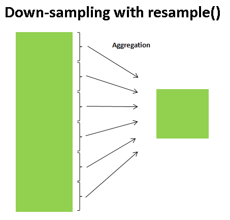![](https://miro.medium.com/max/906/1*60Xzg45SRqJhFueqtOlQ8Q.png) Taking a look at the Google closing price, let's compare what the two return when we **down-sample** the data. Here we will resample the data at the end of business year: ``` goog ``` Date 2014-01-02 554.481689 2014-01-03 550.436829 2014-01-06 556.573853 2014-01-07 567.303589 2014-01-08 568.484192 ... 2015-12-24 748.400024 2015-12-28 762.510010 2015-12-29 776.599976 2015-12-30 771.000000 2015-12-31 758.880005 Name: Close, Length: 504, dtype: float64 ``` # Using resample goog.resample('BA').mean() ``` Date 2014-12-31 559.803290 2015-12-31 602.005681 2016-12-30 NaN Freq: BA-DEC, Name: Close, dtype: float64 ``` # Using asfreq goog.asfreq('BA') ``` Date 2014-12-31 524.958740 2015-12-31 758.880005 Freq: BA-DEC, Name: Close, dtype: float64 ``` goog['2014-12-31'] ``` 524.95874 ``` plt.figure(figsize=(20, 8)) goog.plot(alpha=0.5, style='-') goog.resample('BA').mean().plot(style=':') goog.asfreq('BA').plot(style='--'); plt.legend(['input', 'resample', 'asfreq'], loc='upper left') plt.xticks(rotation=0); ``` How about upsampling? Let's upsample the data to Day. ``` goog[:10] ``` Date 2005-01-03 100.976517 2005-01-04 96.886841 2005-01-05 96.393692 2005-01-06 93.922951 2005-01-07 96.563057 2005-01-10 97.165802 2005-01-11 96.408638 2005-01-12 97.325203 2005-01-13 97.300293 2005-01-14 99.611633 Name: Close, dtype: float64 ``` # Use asfreq to upsample to Day goog.resample('D').mean()[:10] ``` Date 2005-01-03 100.976517 2005-01-04 96.886841 2005-01-05 96.393692 2005-01-06 93.922951 2005-01-07 96.563057 2005-01-08 NaN 2005-01-09 NaN 2005-01-10 97.165802 2005-01-11 96.408638 2005-01-12 97.325203 Freq: D, Name: Close, dtype: float64 ``` goog.asfreq('D')[:10] ``` Date 2005-01-03 100.976517 2005-01-04 96.886841 2005-01-05 96.393692 2005-01-06 93.922951 2005-01-07 96.563057 2005-01-08 NaN 2005-01-09 NaN 2005-01-10 97.165802 2005-01-11 96.408638 2005-01-12 97.325203 Freq: D, Name: Close, dtype: float64 ``` goog.asfreq('D', method='ffill')[:10] ``` Date 2005-01-03 100.976517 2005-01-04 96.886841 2005-01-05 96.393692 2005-01-06 93.922951 2005-01-07 96.563057 2005-01-08 96.563057 2005-01-09 96.563057 2005-01-10 97.165802 2005-01-11 96.408638 2005-01-12 97.325203 Freq: D, Name: Close, dtype: float64 For up-sampling, `resample()` and `asfreq()` are largely equivalent, though resample has many more options available. In this case, the default for both methods is to leave the up-sampled points empty, that is, filled with NA values. Just as with the `pd.fillna()` function , `asfreq()` accepts a method argument to specify how values are imputed. Here, we will resample the business day data at a daily frequency (i.e., including weekends): ``` fig, ax = plt.subplots(2, figsize=(20, 10), sharex=True) data = goog.iloc[:10] data.asfreq('D').plot(ax=ax[0], marker='o') data.asfreq('D', method='bfill').plot(ax=ax[1], style='-o') data.asfreq('D', method='ffill').plot(ax=ax[1], style='--o') ax[1].legend(["back-fill", "forward-fill"]); ``` The top panel is the default: non-business days are left as NA values and do not appear on the plot. The bottom panel shows the differences between two strategies for filling the gaps: forward-filling and backward-filling. ### 3.2 Time Shifting Another common time series-specific operation is shifting of data in time. Pandas has the method `shift()` to computing this. ``` a = goog.asfreq('D', method='ffill')[:10] a ``` Date 2005-01-03 100.976517 2005-01-04 96.886841 2005-01-05 96.393692 2005-01-06 93.922951 2005-01-07 96.563057 2005-01-08 96.563057 2005-01-09 96.563057 2005-01-10 97.165802 2005-01-11 96.408638 2005-01-12 97.325203 Freq: D, Name: Close, dtype: float64 ``` b = goog.asfreq('D', method='ffill').shift(-2)[:10] b ``` Date 2005-01-03 96.393692 2005-01-04 93.922951 2005-01-05 96.563057 2005-01-06 96.563057 2005-01-07 96.563057 2005-01-08 97.165802 2005-01-09 96.408638 2005-01-10 97.325203 2005-01-11 97.300293 2005-01-12 99.611633 Freq: D, Name: Close, dtype: float64 ``` a - b ``` Date 2005-01-03 4.582825 2005-01-04 2.963890 2005-01-05 -0.169365 2005-01-06 -2.640106 2005-01-07 0.000000 2005-01-08 -0.602745 2005-01-09 0.154419 2005-01-10 -0.159401 2005-01-11 -0.891655 2005-01-12 -2.286430 Freq: D, Name: Close, dtype: float64 ``` fig, ax = plt.subplots(2, figsize=(15, 10), sharey=True) # apply a frequency to the data goog = goog.asfreq('D', method='ffill') goog.plot(ax=ax[0]) goog.shift(900).plot(ax=ax[1]) # legends and annotations local_max = pd.to_datetime('2007-11-05') offset = pd.Timedelta(900, 'D') ax[0].legend(['input'], loc=2) ax[0].get_xticklabels()[2].set(weight='heavy', color='red') ax[0].axvline(local_max, alpha=0.3, color='red') ax[1].legend(['shift(900)'], loc=2) ax[1].get_xticklabels()[2].set(weight='heavy', color='red') ax[1].axvline(local_max + offset, alpha=0.3, color='red') plt.show() ``` We see here that `shift(900)` shifts the data by 900 days, pushing some of it off the end of the graph (and leaving NA values at the other end). A common context for this type of shift is in computing differences over time. For example, we use shifted values to compute the one-year return on investment for Google stock over the course of the dataset: ``` # Return on Investment ROI = 100 * ((goog.shift(-365) - goog) / goog) ROI.plot() plt.ylabel('% Return on Investment'); ``` This helps us to see the overall trend in Google stock: thus far, the most profitable times to invest in Google have been (unsurprisingly, in retrospect) shortly after its IPO, and in the middle of the 2009 recession. ### 3.3 Rolling windows Rolling statistics are a third type of time series-specific operation implemented by Pandas. These can be accomplished via the ``rolling()`` attribute of ``Series`` and ``DataFrame`` objects, which returns a view similar to what we saw with the ``groupby`` operation (see [Aggregation and Grouping](03.08-Aggregation-and-Grouping.ipynb)). This rolling view makes available a number of aggregation operations by default. 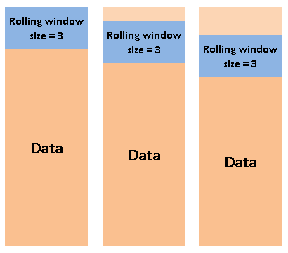![](https://miro.medium.com/max/820/1*jqix0WWK_zDf5iIICpMVjw.png) For example, here is the one-year centered rolling mean and standard deviation of the Google stock prices: ``` goog ``` Date 2005-01-03 100.976517 2005-01-04 96.886841 2005-01-05 96.393692 2005-01-06 93.922951 2005-01-07 96.563057 ... 2015-12-27 748.400024 2015-12-28 762.510010 2015-12-29 776.599976 2015-12-30 771.000000 2015-12-31 758.880005 Freq: D, Name: Close, Length: 4015, dtype: float64 ``` goog.rolling(3).sum() ``` Date 2005-01-03 NaN 2005-01-04 NaN 2005-01-05 294.257050 2005-01-06 287.203484 2005-01-07 286.879700 ... 2015-12-27 2245.200072 2015-12-28 2259.310058 2015-12-29 2287.510010 2015-12-30 2310.109986 2015-12-31 2306.479981 Freq: D, Name: Close, Length: 4015, dtype: float64 ``` rolling = goog.rolling(365, center=True) data = pd.DataFrame({'input': goog, 'one-year rolling_mean': rolling.mean()}) ax = data.plot(style=['-', '--'], figsize=(15,5)) ax.lines[0].set_alpha(0.3) ``` As with group-by operations, the ``.agg()`` and ``.apply()`` methods can be used for custom rolling computations. ## 3. 📖 Further Reading: Time in Python ### 3.1 Built-in library `datetime` Python's basic objects for working with dates and times reside in the built-in `datetime` module. You can use it to quickly perform a host of useful functionalities on dates and times. For example, you can manually build a date using the datetime type: ``` from datetime import datetime datetime(year=2015, month=7, day=4) ``` Once you have a `datetime` object, you can do things like printing the day of the week. The format code can be found at: https://www.programiz.com/python-programming/datetime/strftime ``` date = datetime(year=2015, month=7, day=4) date.strftime('%A') ``` * In the final line, we've used one of the standard string format codes for printing dates ("**%A**"), which you can read about in the `strftime` section of Python's datetime documentation. Documentation of other useful date utilities can be found in `dateutil`'s online documentation. * A related package to be aware of is `pytz`, which contains tools for working with the most migrane-inducing piece of time series data: **time zones**. 🌞 The power of **datetime** and **dateutil** lie in their **flexibility and easy syntax**: you can use these objects and their built-in methods to easily perform nearly any operation you might be interested in. Where they break down is when you wish to work with large arrays of dates and times: just as lists of Python numerical variables are suboptimal compared to NumPy-style typed numerical arrays, lists of Python datetime objects are suboptimal compared to typed arrays of encoded dates. ### 3.2 Time in Numpy: `datetime64` and `timedelta64` https://numpy.org/doc/stable/reference/arrays.datetime.html #### 3.2.1 `datetime64` The weaknesses of Python's datetime format inspired the NumPy team to add a set of native time series data type to NumPy. The `datetime64` dtype encodes dates as **64-bit integers**, and thus allows arrays of dates to be represented very compactly. Also, because of the uniform type in NumPy `datetime64` arrays, this type of operation can be accomplished much more quickly than if we were working directly with Python's datetime objects, especially as arrays get large There are two ways to create a datetime objects in Numpy: * Create a numpy array `dtype=np.datetime64` * Directly create a datetime object by `np.datetime64` ``` import numpy as np date = np.array('2015-07-04', dtype='datetime64') date ``` ``` print(np.array('2015-07-04', dtype='datetime64[D]')) print(np.array('2015-07-04', dtype='datetime64[M]')) print(np.array('2015-07-04', dtype='datetime64[Y]')) print(np.array('2015-07-04', dtype='datetime64[h]')) print(np.array('2015-07-04', dtype='datetime64[m]')) print(np.array('2015-07-04', dtype='datetime64[s]')) ``` Once we have this date formatted, however, we can quickly do vectorized operations on it: ``` date + np.arange(12) ``` Second Method: Directly create a np.datetime object. ``` date = np.datetime64('2005-02-25') date ``` We can force the datetime object to a specific time unit: ``` print(np.datetime64('2005-02-25', 'D')) print(np.datetime64('2005-02-25', 'M')) print(np.datetime64('2005-02-25', 'Y')) print(np.datetime64('2005-02-25', 'h')) print(np.datetime64('2005-02-25', 'm')) print(np.datetime64('2005-02-25', 's')) ``` ``` # Extra: What is Nan in datetime data type? np.datetime64('nat') ``` #### 3.2.2 `timedelta64` The **`timedelta64`** data type was created to complement `datetime64`. The arguments for **timedelta64** are **a number, to represent the number of units, and a date/time unit**, such as (D)ay, (M)onth, (Y)ear, (h)ours, (m)inutes, or (s)econds. The timedelta64 data type also accepts the string “NAT” in place of the number for a “Not A Time” value. ``` # Duration of 1 day np.timedelta64(1, 'D') ``` ``` # Duration of 4 hours print(np.timedelta64(4, 'h')) ``` `Datetimes` and `Timedeltas` work together to provide ways for simple datetime calculations. ``` np.datetime64('2009-01-01') - np.datetime64('2008-01-01') ``` ``` np.datetime64('2009') + np.timedelta64(20, 'D') ``` ``` np.datetime64('2011-06-15T00:00') + np.timedelta64(12, 'h') ``` ``` np.timedelta64(1,'W') / np.timedelta64(1,'D') ``` ``` np.timedelta64(1,'W') % np.timedelta64(10,'D') ``` 💥 **CHALLENGE:** Nhân was born on November 4th 1995, how many minutes has he been living until today? ``` # YOUR CODE HERE ``` ## _References & Beyond_ **Where to Learn More** This section has provided only a brief summary of some of the most essential features of time series tools provided by Pandas; for a more complete discussion, you can refer to the ["Time Series/Date" section](http://pandas.pydata.org/pandas-docs/stable/timeseries.html) of the Pandas online documentation. Another excellent resource is the textbook [Python for Data Analysis](http://shop.oreilly.com/product/0636920023784.do) by Wes McKinney (OReilly, 2012). Although it is now a few years old, it is an invaluable resource on the use of Pandas. In particular, this book emphasizes time series tools in the context of business and finance, and focuses much more on particular details of business calendars, time zones, and related topics.