# Week 14: Learning to See Through Obstructions
###### tags: `技術研討`
* 論文連結：https://arxiv.org/pdf/2004.01180v1.pdf
* 程式碼: [alex04072000/ObstructionRemoval](https://github.com/alex04072000/ObstructionRemoval)
* 官方給的補充資料: https://alex04072000.github.io/ObstructionRemoval/website/ObstructionRemoval-supp.pdf
* PWC-Net: [link](https://arxiv.org/pdf/1709.02371.pdf)
* Demo: [link](https://alex04072000.github.io/ObstructionRemoval/website/Obstruction_HTML_CameraReady/result.html)
* 會議連結：[link](https://meet.google.com/baz-ivxw-uru)

## 1. Introduction (昱睿)
* CVPR 2020 的論文
### :stars: 目的

* 去除圖片中的障礙物：障礙物可能是「反光」、「柵欄、「玻璃上的雨滴等」

### :pushpin: single image
* 近期的研究專注在針對「單一影像檔」移除裡面不想要的反光部分與障礙物，這些方法槓桿了 ghosting cues 以及 learning-based 方法
* **ghosting cues**: ghosting 就是隔著一個玻璃拍照的時候會出現的一些反光區域，[Reflection Removal using Ghosting Cues](http://citeseerx.ist.psu.edu/viewdoc/download?doi=10.1.1.698.7662&rep=rep1&type=pdf)(CVPR-2015) 這篇論文就是用模型建立一個 ghosting model 然後去把它減掉
* ghosting model ([paper link](https://webee.technion.ac.il/~yoav/publications/tReverberate_CVPR.pdf)): 用純數學的方式將 reflection part 以及 tranmission part 算出來 (非 NN)

* **learning-based**: [Single Image Reflection Separation with Perceptual Losses](https://arxiv.org/pdf/1806.05376.pdf) (CVPR-2018) 訓練 GAN 模型去生成指定影像檔的 reflection part 與 transmission part
* 使用合成的 dataset: [fqnchina/CEILNet](https://github.com/fqnchina/CEILNet)
* **小缺點**：如果 testing data 不在訓練資料裡面的話，效果就差很多

### :pushpin: multi-frames
* 為了解決上述問題，multi-frames approach 被提出來，這個方法的特點在影像中的 background 與 occlusion 對攝影機來說會落在不同的深度 (depth)。移動中的相機可以看出來這兩個不同的層之間的 motion difference。缺點：計算量很大，而且需要一些嚴格的假設，例如 assumption of brightness consistancy, assumption of accurate motion estimation
* **brightness consistancy**: 在影像的移動中，現實生活中的同一個點移動前後的 RGB 會一模一樣 ([link](https://www.cc.gatech.edu/~afb/classes/CS4495-Fall2014/slides/CS4495-OpticFlow.pdf))
* **accurate motion estimation**: 假設點移動的估計是準的 (我其實有點找不到，但我是這麼猜測的😂) ([link](https://www.iitr.ac.in/departments/MA/uploads/Lecture%20-%20Optical%20Flow.pdf))

### :pushpin: 本篇特點 (集合以前研究的所有優點)
* model 是純 data-driven 的，而且不需要任何傳統假設 (brightness consistancy, accurate flow fields, planar surface )，這些假設如果成立，可能會導致 reconstuction of layers fail
* 使用合成資料去訓練然後再使用真實資料去 fine-tune 結果效果很好
* 很小的變化卻可以應用在很廣的場域 (在 section 3 會介紹)

## 2. Related Work (立晟、信賢)

### Multi-frame reflection removal
<!-- - [SIFT Flow: Dense Correspondence across Different Scenes](https://www.di.ens.fr/willow/pdfs/liu08.pdf)
- 結合 SIFT 和 Optical Flow

- Image Alignment Problem：輸入一張圖像後，在眾多圖像中找到與之最相像的圖
- 給定一張圖(a)，找出和圖(a)最相似的圖(b)
- Motion Field：
- 圖(c )是從圖(b)得出的 motion field
- 圖(d)是將圖(b)扭曲後，進而得出的 motion field
- 圖(e)是 ground truth -->

- [Robust Separation of Reflection from Multiple Images](https://openaccess.thecvf.com/content_cvpr_2014/papers/Guo_Robust_Separation_of_2014_CVPR_paper.pdf)


- superimposed area (疊加區域) = reflection layer + transmitted layer
- 圖(a)：原圖
- 圖(a)中的藍框：superimposed area (疊加區域)
- 圖(b)：reflection layer
- 圖(c )：transmitted layer

- Priors
- correlation：不同 frame 之間的 transmitted layer 的 correlation 是很高的
- reflection sparsity：reflection layer 相較於 transmitted layer 來說是非常 sparse 的
- gradient sparsity：自然圖像是分段平滑的，所以 gradient 應該是 sparse 的
- gradient independence：transmitted layer 和 reflection layer 的 gradient 應該是彼此獨立的

### Single-image reflection removal
- [Single Image Layer Separation using Relative Smoothnesss](https://openaccess.thecvf.com/content_cvpr_2014/papers/Li_Single_Image_Layer_2014_CVPR_paper.pdf)
- Priors
- reflection layer 較大的 gradients 會比 background layer 少很多 (可以從 gradient histograms 得知)

- [Seeing Deeply and Bidirectionally: A Deep Learning
Approach for Single Image Reflection Removal](https://openaccess.thecvf.com/content_ECCV_2018/papers/Jie_Yang_Seeing_Deeply_and_ECCV_2018_paper.pdf)
- 模型框架
- 3 sub-networks
- 用原圖預測 background layer
- 用原圖和 background layer 預測 reflection layer
- 用原圖和 reflection layer 預測 background layer
- 資料準備
- 隨機選兩張圖並切成很多 patches，最後再組合成一張圖，一張當 reflection，一張當 background

### Occlusion and fence removal

- [ACCURATE AND EFFICIENT VIDEO DE-FENCING USING
CONVOLUTIONAL NEURAL NETWORKS AND TEMPORAL INFORMATION](https://arxiv.org/pdf/1806.10781.pdf)
- 模型框架
- Segmentation：找到 fence 的區域
- Optical Flow：透過光流去 de-fencing
- 資料準備
- 自己架相機，一張拍有柵欄的，一張拍沒有柵欄的

### Video completion
填充影片缺失的合理內容，應用範圍包含去除物體、提高影片穩定度、消除水印等等
- [Temporally coherent completion of dynamic video](https://filebox.ece.vt.edu/~jbhuang/papers/SigAsia_2016_VideoCompletion.pdf)
我們提出了一種自動視頻完成算法，該算法以時間連貫的方式合成視頻中的缺失區域。
- Algorithm pipeline
給定 input video & user-selected mask，並迭代這三個步驟
- 最近臨近區域估計(nearest neighbor field, NNF)：找到最近的像素填補，填補user-selected mask

- 顏色更新
- 光流更新
- Result
### Layer decomposition
我們的方法靈感來自這些層分解方法的開發，特別是在利用物理圖像形成和數據驅動先驗的方法。
- [Learning data-driven reflectance priors for intrinsic image decomposition](https://people.eecs.berkeley.edu/~tinghuiz/papers/iccv15_lrp.pdf)
我們可以很輕易地知道X點和Y點的亮度不同，但是實際上他們來自同一個物體(沙發)。因此我們的分解方式目的是達成X點和Y點也是來自同樣物品，自動地分解和消除反射光線或陰影部分。
- Network for reflectance prediction
the classifier score of same, darker and brighter, respectively
網絡權重是共享的在局部特徵之間，從所有四個管線中提取的特徵通過三個完全連接的層饋送，以進行最終的相對反射率進行預測
- Result
照明條件(例如第 1-3 行)比 Bell 等人的方法，本論文的方法更強調其反射平滑。
- [Inverse Rendering for Complex Indoor Scenes:
Shape, Spatially-Varying Lighting and SVBRDF from a Single Image](https://openaccess.thecvf.com/content_CVPR_2020/papers/Li_Inverse_Rendering_for_Complex_Indoor_Scenes_Shape_Spatially-Varying_Lighting_and_CVPR_2020_paper.pdf)
重建複雜室內場景(可能可應用在線上看房等等？)
- 可以更換材料的質地
- Network
- [Code](https://github.com/lzqsd/InverseRenderingOfIndoorScene)
- [成果影片參考](http://cseweb.ucsd.edu/~viscomp/projects/CVPR20InverseIndoor/github/dataset.mp4)
- [英文講解](https://www.youtube.com/watch?v=RvWlDWtTozw&ab_channel=ComputerVisionFoundationVideos)
### Online optimization
從測試數據中學習一種減少訓練/測試分佈之間域差異的有效方法。 例子包括使用幾何約束、自監督損失、在線模板更新。
- [Self-supervised Learning with Geometric Constraints in Monocular Video Connecting Flow, Depth, and Camera](https://arxiv.org/pdf/1907.05820v1.pdf)
一個用於從單眼相機中學習深度、光流、鏡頭和內在參數的監督式學習框架，本文提出的幾何學習網絡解決了深度預測，光流預測模型，相機內參預測連接的問題。本文提出的幾何學習網絡解決了單眼相機的深度預測、光流預測模型、相機位置、相機內參預測連接的問題。
- Network
該模型可以將連續的圖像幀作為輸入，解決各種任務，例如深度、相機和流量估計，並通過捕獲自適應光度和幾何約束的損失函數將它們耦合。
- Result
- 預測深度
- 預測光流
- [Test-Time Training with Self-Supervision for Generalization under Distribution Shifts](https://arxiv.org/pdf/1909.13231.pdf)
本論文提出了 Test-Time Training，一個提高性能的一般方法訓練和測試數據時的預測模型來自不同的分佈。
- 說明
testing 的時候可以假設有一個x input 去影響了y的長相
我們利用旋轉的方法讓training變成兩種問題，一個是預測角度一個是預測標籤。
在testing的時候我們不知道ｙ，但我們仍然可以最大化loss並劃出新的分佈Q，從原本分佈P去推論x
- [影片講解](https://yueatsprograms.github.io/ttt/home.html)

## 3. Proposed Method (昊中、沛筠)


| 符號 | 說明 |
| - | - |
| $I$, $I_k$ | frame, keyframe |
| $\{I_t\}^T_{t=1}$ | sequence of T frames |
| $B$ | background layer |
| $R$ | reflection layer |
| $L$, $l$ | hierarchy, level |
| $c$ | extracted features |
| $V$ | flow fields |
| $\textbf{W()}$ | bilinear sampling operation |
| $↑_2$, $↓_2$ | upsample 2x, downsample 2x |
| $g_B$ | background reconstruction network |

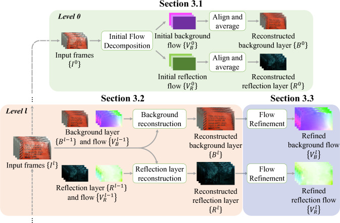
### 3.1. Initial Flow Decomposition :star::star::star:
演算法的初始，必須先將影像分成background與reflection的兩影像。
- 使用方法：透過光流法的應用進行光流的分解。
- 網路架構可分為:
- 一個feature extractor
- 一個layer flow estimator
- feature extractor:
- CV (cost volume): 針對一張frame中的pixel，計算在下一張frame的同位置以及周圍的pixel的之間的相似程度，並作為特徵向量。
<!-- (針對一張image中 的pixel，計算在下一張frame的移動大小) -->
- $CV_{jk}(\text{x}_1, \text{x}_2)=c_j(\text{x}_1)^{\top}c_k(\text{x}_2)$
- $c_j$、$c_k$：frame $j$與$k$的特徵向量
- $\text{x}_1$、$\text{x}_2$：pixel index
- layer flow estimator:
- 以$CV$與$c_j$作為輸入，傳入fully-connected layer產出兩個motion vector(位移向量)。
- 再把兩個向量對應到image上分離出background與reflection。

[參考 1](https://blog.csdn.net/Bruce_0712/article/details/108580474)
[參考 2 (cost volume or correlation volume 解釋)](https://www.aminer.cn/research_report/6086cff030e4d5752f50c847)

### 3.2. Background/Reflection Layer Reconstruction

- 模組的目的在於重建 $B_k$ 及 $R_k$。
- 雖然 background 與 reflection 都是要進行「重建」，但因特性不同，所以是各自訓練 network（結構一樣但不共享參數）。
- 以 background layer reconstruction 為例。


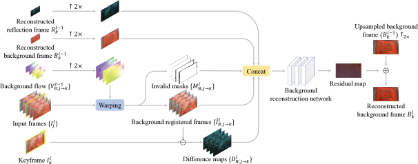
- Level = 0 時，使用 3.1 的方法對齊相鄰的 frames，並計算平均值得到預測的背景圖片。

- $B_k^0=\frac{1}{T}\sum\limits_{j=1}^{T}\textbf{W}(I_j^0, V_{B, j\rightarrow k}^0)$

- $I_j^0$：downsample 到 level 0 的 frame j

- Level = l 時，模型輸入 $B_k^{l-1}$、$R_k^{l-1}$、$\{V_{B, j\rightarrow k}^{l-1}\}$ 和 $\{I_t^l\}$ 來重建 $B_k^l$。

- 先 upsample $\{V_{B, j\rightarrow k}^{l-1})\}$ 2x，接著把所有 $\{I_j^l\}$ 對齊 $\{I_k^l\}$。

- $\widetilde{I}_{B, j\rightarrow k}^l=\textbf{W}(I_j^l, V_{B, j\rightarrow k}^{l-1}↑_2)$

- 遮蔽（occlusion）或超過影像邊界的扭轉（warping）可能會使一些 pixel 失效。為了減少誤差 （artifacts），將計算 difference map（$D_{B, j\rightarrow k}^l=\left | I_{B, j\rightarrow k}^l-I_k^l \right |$）和 warping invalid masks（$M_{B, j\rightarrow k}^l$）。

- 串接已對齊的 frames、difference maps、invalid masks 和 upsampled 的前層 background 及 reflection layers 並輸入 network 得到 $I_k^l$ 的預測 residual map，再把 residual map 與 $(B_k^{l-1})↑_2$ 相加即為 $B_k^l$。

- $B_k^l=g_B(\{\widetilde{I}_{B, j\rightarrow k}^l\}, \{D_{B, j\rightarrow k}^l\}, \{M_{B, j\rightarrow k}^l\}, (B_k^{l-1})↑_2, (R_k^{l-1})↑_2)+(B_k^{l-1})↑_2$

### 3.3. Optical Flow Refinement (PWC-Net)
使用pre-trained的PWC-Net針對重建完成的image進行光流的細部修正。
- PWC-Net
- 透過 Feature Pyramid, Warping, Cost Volume 去計算兩張影像之間的光流
- 本篇論文的PWC模型的使用上，不會去更新模型，僅用來作為細部光流的修正。

### 3.4. Network Training
- 採用two-stage training:
- 1.訓練initial flow decomposition網路
- $\mathcal{L}_{\text{dec}}=\sum\limits_{k=1}^T{\sum\limits_{j=1,j\not=k}^T{\Vert{V_{B,j\to{k}}^0}-\text{PWC}(hat{B_j},\hat{B_k})\downarrow^{2^{L}}\Vert_{1}+\\\Vert{V_{R,j\to{k}}^0}-\text{PWC}(hat{R_j},\hat{R_k})\downarrow^{2^{L}}\Vert_{1}}}$
- 2.訓練layer reconstruction網路
- $\mathcal{L}_{\text{img}}=\frac{1}{T \times L}\sum\limits_{t=1}^T\sum\limits_{l=0}^L(\Vert\hat{B_t^l}-{B_t^l}\Vert_1+\Vert\hat{R_t^l}-{R_t^l}\Vert_1)$
- $\mathcal{L}_{\text{grad}}=\frac{1}{T \times L}\sum\limits_{t=1}^T\sum\limits_{l=0}^L(\Vert\nabla\hat{B_t^l}-\nabla{B_t^l}\Vert_1+\Vert\nabla\hat{R_t^l}-\nabla{R_t^l}\Vert_1)$
- $\mathcal{L}=\mathcal{L}_{\text{img}}+\lambda_{grad}\mathcal{L}_{\text{grad}}$
### 3.5 Synthetic Sequence Generation (合成連續影像)
蒐集具有ground truth的真實影像很困難，所以採用兩個連續影像疊加，一個作為background，一個作為reflection。

### 3.6. Online Optimization

- 利用真實影像 finetune 模型。

- unsupervised warping consistency loss：使預測的 background 和 reflection layers 在 warped back 且重組後等同原始影像。
- $\mathcal{L}_{\text{warp}}=\sum\limits_{k=1}^T\sum\limits_{j=0, j\neq k}^T\sum\limits_{l=0}^L\Vert I_j^l-(\textbf{W}(B_k^l, V_{B, j\rightarrow k}^l)+(\textbf{W}(R_k^l, V_{B, j\rightarrow k}^l)) \Vert_1$

- total variation loss
- $\mathcal{L}_{tv}=\sum\limits_{t=1}^T\sum\limits_{l=0}^L(\Vert\nabla B_t^l\Vert_1+\Vert\nabla R_t^l\Vert_1)$

- overall loss of online optimization
- $\mathcal{L}_{online}=\mathcal{L}_{\text{warp}}+\lambda_{tv}\mathcal{L}_{tv}$

### 3.7 Extension to Other Obstruction Removal (實現其他障礙物的移除)

- 提出的 framework 在簡單修改後，可以應用至其他問題，並獲得不錯的效果。

1. 移除 reflection 重建架構，只保留 background 部分。
2. 增加新的分支在 background 重建架構的輸出處來分割障礙物。
- 估算的 network 無法很好的處理重複結構（圍籬）與微小物件（雨滴），因此經常產生 noisy 的光流。

## 4. Experiments and Analysis (昱睿)
### 4.1. Comparisons with State-of-the-arts
* 量化評估指標
* (**$\uparrow$**) PSNR (峰值訊噪比, Peak signal-to-noise ratio): 經常用於衡量圖片壓縮後的結果。數字越高代表看得出來兩圖的差異；數字越低的意思就是看不出來兩圖有什麼差別，也就是感覺好像沒改變
* (**$\uparrow$**) SSIM (Structural SIMilarity): 訊號相似度 : [paper link](https://www.cns.nyu.edu/pub/lcv/wang03-preprint.pdf)
* (**$\uparrow$**) NCC (Normalized cross correlation): 用衡量兩張圖片有多像。以下為公式，$f,\, t$ 是兩個影像檔 (假設 shape 一樣，都是 $N$)，$\sigma_f$ 代表 f 這張圖片 pixel 的 variance。[wiki link](https://en.wikipedia.org/wiki/Cross-correlation)
$$
NCC=\frac{1}{N}\times \sum_{x,\, y}\frac{1}{\sigma_f \, \sigma_t}(f(x, y) + t(x, y))
$$
* (**$\downarrow$**)LMSE (local mean squared error): 就是把 A, B 兩張影像檔用 local 的方式掃過，加總所有的 MSE。 local 的意思是用 k $\times$ k 的 window 去擷取，每次的步伐是 $\frac{k}{2}$ 步。目的在計算 2 個影像之間的 local 誤差總和
$$
LMSE(A, B)=\sum_{\omega \in W}MSE(A_\omega, B_\omega)
$$

$$
MSE(A, B) = min_{\alpha}(||A - \alpha B||^2)
$$
* :star: 實驗一：controlled sequences: 使用 [42] 號論文提供的資料，下面的數據都是使用 $NCC$ 來評估
---
* :star: 實驗二：Synthetic sequences - 用 100 個 sequences of images 去測，每個 sequence of images 是 5 張圖片，如果是針對 single image 的 model，就使用 5 張一樣的圖片去測試
---
* :star: 實驗三：Real sequences

### 4.2. Analysis and Discussion

#### :star: Initial flow decomposition.

* 一開始的均勻 flow 設定是很重要的，跟一開始 flow 都是 0 的 case 相比， uniform 的模型在 validation loss 低多了

#### :star: Image reconstruction network.

* 影像重建方式改用 temporal filtering 再加上用光流混合附近影像檔的方式，結果誤差變很大
* temporal filtering 是一種用 Fourier Transform 的方式去雜訊: [link](https://en.wikibooks.org/wiki/Neuroimaging_Data_Processing/Temporal_Filtering)

#### :star: Online optimization.

* pre-trained model 以及 online fine-tune 缺一不可

#### :star: Failure case.

* reflection layer 有兩層的話就會失敗

## 5. Conclusions (昱睿)

* 整篇看下來我覺得這篇滿厲害的，後續還可以做的應該就是解決失敗照片那邊，如果主要物品被多重 obstruction 遮住的話，要如何解決

## 6. 可能的應用方式

* 在申請流程中請顧客開啟 app 使用相機拍照，在拍照的過程中收集「影片」，此時即將模型針對收集的影片做 inference 並存下較清晰的照片


## 7. 補充
### 2. Related Work
#### Video completion
- [A Survey on Data-Driven Video Completion](https://ur.booksc.org/book/57890821/60521b)
如何實作的示意圖：
- Pixel and Patch-Based Completion
在每次迭代中，首先初始化最近鄰域 (NNF)；該字段包括孔中每個目標補丁的最接近匹配補丁。
- Object-Based methods
- Template-basedmethods
(左圖)利用背景減法(假設靜止相機和靜態背景)，分割過程將多個對象相互分離，並將對像模板（對象移動的簡短片段）存儲到數據庫中以備後用。 使用來自時間偏移的資訊修復缺失的靜態背景區域。
- Explicithumanmodelling
(右圖)一種基於輪廓的方法來完成被遮擋的對象。首先，對視頻中的運動物體進行分析，提取出物體的姿態以備後用。姿勢經過關鍵姿勢選擇階段，在該階段選擇、保存和標記具有代表性的姿勢。在下一步中，構建虛擬輪廓。這些稍後將用於指導後面的姿勢位置。
- Lighting Corrections
Poisson image blending是一種流行的無縫圖像複製工具，梯度域混合的使用恢復了該區域中的目標顏色，以解決目標照明差異。
#### Layer decomposition
- [Flash Photography Enhancement via Intrinsic Relighting](https://people.csail.mit.edu/fredo/PUBLI/flash/flash.pdf)
由於在比較暗的場景，攝影師會考慮使用閃光燈，但可能會過度曝光、紅眼、陰影不正常。本論文會藉由一張暗圖片和閃光圖片來重建影像的陰影。
#### Online optimization
- [Tracking-Learning-Detection](http://vision.stanford.edu/teaching/cs231b_spring1415/papers/Kalal-PAMI.pdf)
TLD 追踪系統最大的特點就在於能夠對鎖定的進行不斷的學習，以獲取目標最新的外觀特徵，從而改進及時追踪，達到最佳的狀態。隨著目標的不斷運動，系統能夠持續不斷地進行探測，獲知目標在角度、距離、景深等方面的變化，並實時識別，經歷了重點的學習之後，目標就再也無法躲過 。
TLD 算法由三部分組成：跟踪模塊、檢測模塊、學習模塊。跟踪模塊是觀察幀與幀之間的目標的動向。模塊是把每張圖看成獨立的，然後去定位。學習模塊將根據追踪模塊的結果對檢測模塊的錯誤進行評估，生成訓練樣本來對檢測模塊的模型進行更新，避免以後出現類似錯誤。
- P-N Learning
我們希望在每一幀都對當前檢測器進行評估，識別錯誤，更新讓未來減少錯誤。
思想核心是：P-專家識別漏檢（假陰性），N-專家識別誤檢（假陽性）。PN學習主要幾個模塊組成：
- (1)學習過的分類器
- (2)訓練集：得到以下一組標記過的訓練樣本
- (3)監督訓練：從訓練集上訓練分類器的一個方法
- (4)PN專家：在學習過程中產生正負樣本的函數。其流程如下：

<!-- https://www.gushiciku.cn/pl/gVvu/zh-hk -->