---
tags: Algorithm
---
<style>
font {
color: red;
font-weight: bold;
}
</style>
# Ch02 - Divide and Conquer
- Methodology of Divide-and-Conquer
- Top-Down Approach
- Divide an instance of a problem into two or more **smaller instances**
$\Rightarrow$ which are **usually instances of the original problem**
- If solutions to the smaller instances can be obtained readily
$\Rightarrow$ **the solution** to the original instance can be obtained by **combining these solutions**.
- If the smaller instances are still too large to be solved readily
$\Rightarrow$ they can be **divided into still smaller instances**.
- the process continues until they are so small that a solution is readily obtainable.)
- **Recursion** $\rightarrow$ **Iteration**
- When we developing a Divide-and-Conquer algorithm, we usually think at problem-solving level and write it as a recursive routine.
- Then, we can create a **more efficient iterative version** of the algorithm. (E.g., using DP, Dynamic Programming)
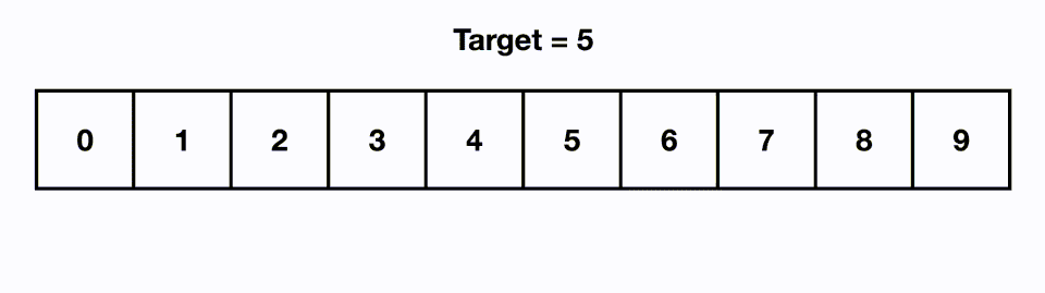
## Binary Search
- **Goal**: determine whether $x$ is in the **sorted array** $S$ of $n$ keys.
- **Steps**:
1. If $x$ equals the **middle item**, quit.
2. Divide the array into two subarrays about **half** as large. If $x$ < middle item, choose the left subarray, otherwise, the right.
3. Use **recursion** to conquer the subarray until find $x$ or not in the array.
### Binary Search (Recursive)
Determine whether `x` is in the sorted array `S` if size `n`.
> **Input:** positive integer `n`, sorted (nondecreasing order) array of keys `S` indexed from `1` to `n`, a key `x`.
> **Output:** `location`, the location of `x` in `S` (0 if `x` is not in `S`)
```cpp=
index location (index low, index high) {
index mid;
if (low > high) return 0;
else {
mid = low + (high - low) / 2;
if (x == S[mid]) return mid;
else if (x < S[mid]) return location(low, mid-1);
else return location(mid+1, high);
}
}
```
### Complexity Analysis
Since it has *no every-case* time complexity, we do the *worst-case* analysis
- **Worst-Case Time Complexity**
- For *searching algorithms*, the most costly operation is usually the **comparison**
- **Basic Operation**: the comparison of $x$ with $S[mid]$
- **Input Size**: $n$, the number of items in the array
- The worest case occurs when $x$ is not in $S$ ($x$ is larger than all the items).
- Each recursive call will **halve** the instance when $n = 2^m$
$$
W(n) = W(\frac{n}{2}) + 1
$$
> $+1$: the comparision at top level
- Because $W(1)=1$, the solution is:
$$
W(n) = \lfloor \lg n \rfloor + 1
$$
## Merge Sort
- **Steps**:
1. Divide the array into two subarrays each with $n/2$ items.
2. Conquer each subarray by sorting it.
- Unless the array is sufficiently small, use recursion to do this.
3. Combine the solution to the subarray by merging them into a single sorted array.

### Merge Sort
Sort `n` keys in nondecreasing sequence.
> **Input:** positive integer `n`, array of keys `S` indexed from `1` to `n`.
> **Output:** the array `S` containing the keys in nondecreasing order.
```cpp=
void mergesort (int n, keytype S[]) {
if (n > 1) {
const int h = floor(n/2), m = n - h;
keytype U[1..h], V[1..m];
copy S[1] through S[h] to U[1] through U[h];
copy S[h+1] through S[n] to V[1] through V[m];
mergesort(h, U);
mergesort(m, V);
merge(h, m, U, V, S);
}
}
```
### Merge
Merge two sorted arrays into one sorted array.
> **Input:** positive integers `h` and `m`, array of sorted keys `U` indexed from `1` to `h`, array of sorted keys `V` indexed from `1` to `m`.
> **Output:** an array `S` indexed from `1` to `h+m` containing the keys in `U` and `V` in a single sorted array.
```cpp=
void merge (int h, int m, const keytype U[],
const keytype V[],
const keytype S[]) {
index i, j, k;
i = 1; j = 1; k = 1;
while (i <= h && j <= m) {
if (U[i] < V[j]) {
S[k] = U[i];
i++;
} else {
S[k] = V[j];
j++;
}
k++;
}
if (i > h) {
copy V[j] through V[m] to S[k] through S[h+m];
} else {
copy U[i] through U[h] to S[k] through S[h+m];
}
}
```

### Improved version
- **In-place sort** is a sorting algorithm that **does not use any extra space** beyond that needed to store the input.
### mergesort 2 (improved version)
Sort `n` keys in nondecreasing sequence.
> **Input:** positive integer `n`, array of keys `S` indexed from `1` to `n`.
> **Output:** the array `S` containing the keys in nondecreasing order.
```pseudo=
void mergesort2 (index low, index high) {
index mid;
if (low < high) {
mid = low + ⌊ (high - low) / 2 ⌋ ;
mergesort2(low, mid);
mergesort2(mid+1, high);
merge2(low, mid, high);
}
}
```
### merge 2 (improved version)
Merge the two sorted subarrays of `S` created in Mergesort2.
> **Input:** indices `low`, `mid`, and `high`, and the subarray of `S` indexed from `low` to `high`.
> **Output:** the subarray of `S` indexed from `low` to `high` containing the keys in nondecreasing order.
```pseudo=
void merge2(index low, index mid, index high) {
index i, j, k;
keytype U[low..high]; // A local array needed for the merging
i = low, j = mid + 1, k = low;
while (i <= mid && j <= high) {
if (S[i] < S[j]) {
U[k] = S[i];
i++;
} else {
U[k] = S[j];
j++;
}
k++;
}
if (i > mid)
move S[j] through S[high] to U[k] through U[high];
else
move S[i] through S[mid] to U[k] through U[high];
move U[low] through U[high] to S[low] through S[high];
}
```
## Divide and Conquer
The <font>*divide and conquer*</font> design strategy involves the following steps:
- <font>*Divide*</font> an instance of a problem into one or more smaller instances.
- <font>*Conquer*</font> (solve) each of the smaller instances. Unless a smaller instance is sufficiently small, use recursion to do this.
- If necessary, <font>*combine*</font> the solutions to the smaller instances to obtain the solution to the original instance.
## Quicksort
### Steps
- **Pivot**
* to be used to partition the array by Pivot (items smaller than pivot, items larger than pivot)
* it can be any item, and for convenience we use the first item in the input array.
- The **partition** procedure is continued until an array with one item is reached.
- Worst Case:$Ο(n^2)$
- 當資料的順序恰好為由大到小或由小到大時
- 有分割跟沒分割一樣
### Quicksort
Sort `n` keys in nondecreasing order.
> **Input:** positive integer `n`, array of keys `S` indexed from `1` to `n`.
> **Output:** the array `S` containing the keys in nondeceasing order.
```pseudo=
void quicksort (index low, index high) {
index pivotpoint;
if (high > low) {
partition(low, high, pivotpoint);
quicksort(low, pivotpoint-1);
quicksort(pivotpoint+1, high);
}
}
```
### Partition
Partition the array `S` for quicksort.
> **Input:** two indices, `low` and `high`, and the subarray of `S` indexed from `low` to `high`.
> **Output:** `pivotpoint`, the pivot point for the subarray indexed from `low` to `high`.
```cpp=
void partition(index low, index high, index& pivotpoint) {
index i, j;
keytype pivotitem;
pivotitem = S[low]; // Choose first item for pivotitem.
j = low;
for (i=low+1; i<=high; i++) {
if (S[i] < pivotitem) {
j++;
exchange S[i] and S[j];
}
}
pivotpoint = j;
exchange S[low] and S[pivotpoint];
}
```

:::success
**Partition** 的目的是把 array 整理成
- $pivot$ 的左邊都比 $pivot$ 小
- $pivot$ 的右邊都比 $pivot$ 大
可以有幾種做法:
- 把比 $p$ 小的往左邊拉 (演算法課本)
- 把比 $p$ 大的往右邊拉
- 以上兩種同時做 (資結課本)
所以上面的程式碼中:
- `i`: 從左到右看過整個陣列,如果 `S[i] < pivotitem` 就進行交換
- `j`: 和 `S[i]` 交換的位置
- 因為 `S[i]` 要被換到靠左的位置
- 所以 `j` 會從最左邊開始往右跑
- 這樣可以保證最後在 `pivotitem` 左邊的都會比 `pivotitem` 小
:::
## Strassen’s Matrix Multiplication
:::info
**Ex2.4**
Suppose we want the product C of two $2 \times 2$ matrices, *A* and *B*. That is,
$$
\begin{bmatrix}
c_{11} & c_{12} \\
c_{21} & c_{22} \\
\end{bmatrix} =
\begin{bmatrix}
a_{11} & a_{12} \\
a_{21} & a_{22}
\end{bmatrix} \times
\begin{bmatrix}
b_{11} & b_{12} \\
b_{21} & b_{22}
\end{bmatrix}
$$
Strassen determined that if we let
$$
\begin{split}
&m_1 = (a_{11} + a_{22})(b_{11} + b_{22}) \\
&m_2 = (a_{21} + a_{22})b_{11} \\
&m_3 = a_{11}(b_{12} - b_{22}) \\
&m_4 = a_{22}(b_{21} - b_{11}) \\
&m_5 = (a_{11} + a_{12})b_{22} \\
&m_6 = (a_{21} - a_{11})(b_{11} + b_{12}) \\
&m_7 = (a_{12} - a_{22})(b_{21} + b_{22}), 累死
\end{split}
$$
the product C is given by
$$
C = \
\begin{bmatrix}
m_1 + m_4 - m_5 + m_7 & m_3 + m_5 \\
m_2 + m_4 & m_1 + m_3 - m_2 + m_6
\end{bmatrix}
$$
:::
### Partitioning into Submatrices in Strassen’s Algorithm
$$
\begin{bmatrix}
C_{11} & C_{12} \\
C_{11} & C_{12}
\end{bmatrix} =
\begin{bmatrix}
A_{11} & A_{12} \\
A_{11} & A_{12}
\end{bmatrix} \times
\begin{bmatrix}
B_{11} & B_{12} \\
B_{11} & B_{12}
\end{bmatrix}
$$
> $A_{ij}, B_{ij}, C_{ij}$ are $\frac12 \times \frac12$ submatrices
Using Strassen's methid, we first compute
$$
\begin{split}
&M_1 = (A_{11} + A_{22})(B_{11} + B_{22}) \\
&M_2 = (A_{21} + A_{22})B_{11} \\
&M_3 = A_{11}(B_{12} - B_{22}) \\
&M_4 = A_{22}(B_{21} - B_{11}) \\
&M_5 = (A_{11} + A_{12})B_{22} \\
&M_6 = (A_{21} - A_{11})(B_{11} + B_{12}) \\
&M_7 = (A_{12} - A_{22})(B_{21} + B_{22})
\end{split}
$$
Next we compute:
$$
\begin{split}
C_{11} =& M_1 + M_4 - M_5 + M_7 \\
C_{12} =& M_3 + M_5 \\
C_{21} =& M_2 + M_4 \\
C_{22} =& M_1 + M_3 - M_2 + M_6 \\
\end{split}
$$
:::info
**Exp**
$$
A = \begin{bmatrix}
1 & 2 & 3 & 4 \\
5 & 6 & 7 & 8 \\
9 & 1 & 2 & 3 \\
4 & 5 & 6 & 7
\end{bmatrix} \
B = \begin{bmatrix}
8 & 9 & 1 & 2 \\
3 & 4 & 5 & 6 \\
7 & 8 & 9 & 1 \\
2 & 3 & 4 & 5
\end{bmatrix}
$$
$$
\begin{split}
\end{split} \\
\begin{split}
M_1 &= (A_{11} + A_{22})(B_{11} + B_{22}) \\
&= \left(
\begin{bmatrix}
1 & 2 \\ 5 & 6
\end{bmatrix} +
\begin{bmatrix}
2 & 3 \\ 6 & 7
\end{bmatrix}
\right) \times
\left(
\begin{bmatrix}
8 & 9 \\ 3 & 4
\end{bmatrix} +
\begin{bmatrix}
9 & 1 \\ 4 & 5
\end{bmatrix}
\right) \\
&= \begin{bmatrix}
3 & 5 \\ 11 & 14
\end{bmatrix} \times
\begin{bmatrix}
17 & 10 \\ 7 & 9
\end{bmatrix} =
\begin{bmatrix}
86 & 75 \\ 278 & 227
\end{bmatrix}
\end{split}
$$
:::
### Strassen’s Matrix Multiplication
Determine the product of two $n \times n$ matrices where $n$ is a power of $2$
> **Inputs**: ab interger $n$ that is a power of $2$, and two $n \times n$ matrices $A$ abd $B$
> **Output**: the product $C$ of $A$ and $B$
## Master Theorem
Assume that there are $a$ subproblems, each of size 1/$b$ of the original problem, and that the algorithm used to combine the solutions of the subproblems runs in time $cn^k$, for some constants $a$, $b$, $c$, and $k$. The running time $T(n)$ of the algorithm thus satisfies
$$
T(n) = aT(n/b) + cn^k
$$
We assume, for simplicity, that $n = b^m$, so that $n/b$ is always an integer(b is an integer greater than 1).
Expand the recurrence equation a couple of times
$$
\begin{split}
T(n) =& aT(n/b) + cn^k \\
=& a(aT(n/b^2) + c(n/b)^k)+cn^k \\
=& a(a(aT(n/b^3) + c(n/b^2)^k)+c(n/b)^k)+cn^k
\end{split}
$$
In general, if we expand all the way to $n/b^m=1$, we get
$$
T(n) = a(a(... T(n/b^m)+c(n/b^{m- 1})^k) + ...)+cn^k
$$
Assume the $T(n/b^m)=T(1)=c$. Then
$$
T(n)=ca^m + ca^{m-1}b^k + ca^{m-2}b^{2k} +...+ cb^{mk}
$$
which implies that
$$
T(n) = c\displaystyle\sum_{i=0}^{m}a^{m-i}\ b^{ik} = ca^m\displaystyle\sum_{i=0}^{m}({b^k \over a})^i
$$
The solution of the recurrence relation , where $a$ and $b$ are integer constants, $a \ge 1$, $b \ge 2$ and $c$ and $k$ are positive constants, is
$$
T(n) =
\begin{cases}
O(n^{\log_b a})&\text{if}\ a\!>\!b^k \\
O(n^k{\log n})&\text{if}\ a\!=\!b^k \\
O(n^k)&\text{if}\ a\!<\!b^k \\
\end{cases}
$$
:::success
**EXAMPLE**
Consider the recurrence
$$
T(n) = 9T(\frac n3) +n.
$$
$a = 9$, $b = 3$ and $k = 1$, then $a > b^k \Rightarrow 9 > 3^1 = 3$, use
**case 1:** $\log_b a = 2 \Rightarrow n^{\log_b a} = n^2 \Rightarrow T(n) = \Theta(n^2)$.
:::
:::success
**EXAMPLE**
Consider the recurrence
$$
T(n) = 27T(\frac n3) +n^3.
$$
$a = 27$, $b = 3$ and $k = 3$, then $a = b^k \Rightarrow 27 = 3^3$, use
**case 2:** $n^k{\log n} = n^3 \log n \Rightarrow T(n) = \Theta(n^3 \log n)$.
:::
:::success
**EXAMPLE**
Consider the recurrence
$$
T(n) = 2T(\frac n2) +n^2.
$$
$a = 2$, $b = 2$ and $k = 2$, then $a = b^k \Rightarrow 2 < 2^2 = 4$, use
**case 3:** $n^k = n^2 \Rightarrow T(n) = \Theta(n^2)$.
:::
 Sign in with Wallet
Connect another wallet
Sign in with Wallet
Connect another wallet