# variational autoencoders: a brief introduction with clear notation

## introduction

So you've heard the terms "variational inference", "autoencoder", and "variational autoencoder" thrown around. What are these, what problems do they solve, and how do they relate to each other?

Here's the high-level problem setting before diving into the math. For all three problems, we observe some variables $X$. We assume that there are some hidden **latent variables** $Z$ that are "responsible" for these images in some sense. (In terms of graphical models, this is just two nodes $X$ and $Z$ with an arrow from $Z \to X$.) Let $\mathcal{X}$ and $\mathcal{Z}$ denote the spaces they're supported over. Here's the summary of what these three terms mean:

1. **Variational inference**: a general class of methods for approximating the posterior $\Pr(Z \mid X)$ through optimization. We typically seek to minimize the "difference" between our model and the true posterior, often by equivalently maximizing the "evidence lower bound". Variational autoencoders are one such method.
2. **Autoencoders**: _deterministically_ compressing $X$ into a lower-dimensional $Z$.
3. **Variational autoencoders**: _probabilistically_ compressing $X$ into a lower-dimensional $Z$ where the space $\mathcal{Z}$ has _additional structure_ that allows for _generative modelling_. We optimize the parameters of an **encoder** and **decoder** to maximize the evidence lower bound.

I haven't explained what the "evidence lower bound" is, or what I mean by "additional structure", so if you're curious, read on!

**Motivating example**: $X \in \mathcal{X} = \{ 0, 1 \}^{28 \times 28}$ is an image from MNIST, i.e. a black-and-white image of a digit from $0$ to $9$, and $Z \in \mathcal{Z} = \mathbb{R}^2$ is a two-dimensional latent vector.

## clarifications and notation

One of the challenges I faced when learning about variational inference was understanding the (often unclear) notation. It was challenging to tell which parameters were being used for which functions, and which probabilities were "true" probabilities and which ones were being modelled. Here, I'll use the following notation, aimed at making such distinctions more clear.

- $\Pr$ to represent the _unknown_ true probability measure on the probability space on which $X$ and $Z$ are defined;
- $\mathcal{X}$ for the $|\text{input}|$-dimensional support of $X$;
- $\mathcal{Z}$ for the $|\text{latent}|$-dimensional support of $Z$;
- $\Delta(\mathcal{A})$ for the space of distributions over some set $\mathcal{A}$;
- $\mathcal{F}_{Z} \subset \Delta(\mathcal{Z})$ for a parameterized distribution family (chosen by us) over $\mathcal{Z}$. Let $\Omega$ denote its parameter space;
- $\mathcal{F}_{X} \subset \Delta(\mathcal{X})$ (ditto for $\mathcal{X}$). Let $\Psi$ denote its parameter space;
- $\Pr(Z \mid x)$ to represent the _distribution_ of $Z$ given $X = x$, and $\Pr(z \mid x)$ for its _density_ at a given point $z \in \mathcal{Z}$ (and similar notation for other distributions);
- $\pi(Z)$ for our chosen "prior" distribution over $\mathcal{Z}$. Note that we get to choose this; it's _different_ from the true marginal distribution $\Pr(Z)$.
- $q_{\phi}$ for the **encoding** map from $\mathcal{X}$ to $\mathcal{Z}$ that depends on hyperparameters $\phi$;
- $p_{\theta}$ for the **decoding** map from $\mathcal{Z}$ to $\mathcal{X}$ that depends on hyperparameters $\theta$;
- In the probabilistic case, $q_{\phi}[x](z)$ and $p_{\theta}[z](x)$ for the respective density functions (see below).

**A note on parameterized distribution families**: In variational autoencoders, $q_{\phi}$ and $p_{\theta}$ map to _distributions_ over their respective codomains. Let's make this concept more concrete: for the decoder $q_{\phi}$, once we've chosen $\mathcal{F}_{Z}$, we can instead think of $q_{\phi}$ as being a map $\tilde q_{\phi} : \mathcal{X} \to \Omega$ to the _parameters_ that pick out a distribution from the family. The same goes for the encoder: after choosing $\mathcal{F}_{X}$, then $p_{\theta}$ is equivalent to a map $\tilde p_{\theta} : \mathcal{Z} \to \Psi$. (Apologies for Greek alphabet soup!)

- For our MNIST example, if we choose $\mathcal{F}_{Z}$ to be the isotropic bivariate Gaussian distribution family parameterized by $(\mu, \sigma) \in \Omega = \mathbb{R}^{2} \times \mathbb{R}^{2}$, then $\tilde q_{\phi} : x \mapsto (\mu, \sigma)$, from which we can then evaluate $q_{\phi}[x](z) = \mathcal{N}(z ; \mu, \sigma)$. For the decoder, we could choose $\mathcal{F}_{X}$ to be the family where each pixel is a Bernoulli trial. Then $\Psi = [0, 1]^{28 \times 28}$ and $\tilde p_{\theta} : z \mapsto Y$, a $28 \times 28$ matrix containing the probabilities for each trial. Note that in this particular case, $\Psi = \mathcal{X}$, allowing us to easily visualize the decoded output.

Sampling from these distributions is typically notated by something like $z \sim q_{\phi}(\cdot \mid x)$ and $x \sim p_{\theta}(\cdot \mid z)$. However, here I'll use the notation $q_{\phi}[x](z)$ and $p_{\theta}[z](x)$ for the corresponding density functions and $q_{\phi}[x](Z)$ and $p_{\theta}[z](X)$ for the corresponding distributions. I like this notation better since it reads from left-to-right and better matches the implementation. Hopefully this makes things less ambiguous, but if you feel that I'm committing a total atrocity, let me know.

Keep in mind that in our setting, the hyperparameters $\phi, \theta$ are *not* stochastic, *nor* are they fixed: rather, they get *optimized* over the course of the training procedure. (That being said, Appendix F of the original VAE paper describes a method for including them in the process of variational inference, but we won't delve into that here.)

## slightly more in-depth overview

### variational inference

**Variational inference** aims to tackle the problem: given an observation $x,$ can we calculate the *posterior distribution* $\Pr(Z \mid x)$? This is an example of statistical inference; given an observation, we seek to learn about the distribution it came from.

- Ideally, we'd use Bayes' rule to calculate this. The issue with Bayes' rule is that we need to calculate the normalizing constant in the denominator, $\sum_{z \in \mathcal{Z}} \Pr(x \mid z) \Pr(z),$ which is often impossible or computationally intractable for complex or high-dimensional distributions.
- Instead, we'll *approximate* this distribution by choosing some parameterized distribution family, using $q_{\phi}[x](Z)$ to model $\Pr(Z \mid x)$. This lets us optimize over the hyperparameters $\phi$ to get as "close" to the desired distribution as possible in terms of (reverse) KL divergence.
- It turns out that minimizing the KL divergence is equivalent to maximizing the "evidence lower bound" (ELBO), which we'll describe later. Calculating the ELBO requires access to the likelihood $\Pr(X \mid z)$; if we don't have access to it, then instead we can model it with a decoder $p_{\theta}$, and the system as a whole is called a "variational autoencoder" for reasons that will soon become obvious.
- Now we can use our model of the posterior for any desired purpose! For example, suppose $Z$ is the binary variable indicating whether $X$ is an image of my cat Mochi. Then $q_{\phi}[x](Z) \in \mathcal{F}_{Z}$ can be parameterized by just a single parameter $p \in \Omega = [0, 1]$ indicating the predicted probability that $x$ is a picture of Mochi.
- This is an optimization-based alternative to traditional sampling-based methods for posterior approximation such as Markov Chain Monte Carlo (MCMC).

### autoencoders

For **autoencoders**, which are built on fully *deterministic* processes, we'll set up a very different relationship between $X$ and $Z.$ Specifically, given $x,$ we want $z$ to be a low-dimensional "compressed version" of $x$ that we calculate using the encoder $q_{\phi}: \mathcal{X} \to \mathcal{Z}.$ What are we optimizing for, specifically? Well, we want $Z$ to contain "as much information" about $X$ as possible, so that for a given $z,$ we can *recreate* the original input $X$ using the decoder $p_{\theta}: \mathcal{Z} \to \mathcal{X}.$ Ideally, for any $x,$ we'd like $p_{\theta}(q_{\phi}(x)) \approx x.$ We'll optimize over the hyperparameters $\theta, \phi$ to make the "difference" (measured by some loss function) between the two sides of that equation as small as possible. (Note that the term "hyperparameter" is a little useless in this case since there's no "ground-level" parameters, but I'll stick with it for consistency.)

- This is all I'll say about autoencoders for the moment; see [Lilian Weng's blog post](https://lilianweng.github.io/posts/2018-08-12-vae/) for more details.

### variational autoencoders

**Variational autoencoders** combine both of the above techniques, and are more general than autoencoders in a certain sense. Consider the following: what if I want to generate additional images that are similar to a given image $x$?

- Using autoencoders, we might try to randomly sample vectors from the latent space and pass these through the decoder. However, there might be large areas of the latent space that don't correspond to any inputs $x$; we'd need to visualize a _lot_ of the space to find the important patches. In other words, it's unclear that the optimization process will lead to a "continuous" latent space.
- Variational autoencoders address this problem and allow for *generative modelling* by using _regularization_ to enforce a certain structure over the latent space. The key difference is that we make the encoder and decoder *stochastic*. The encoder (aka "discriminative model") $q_{\phi}$ now maps from $\mathcal{X}$ to *distributions* over $\mathcal{Z},$ and the decoder (aka "generative model") $p_{\theta}$ maps from $\mathcal{Z}$ to *distributions* over $\mathcal{X}.$ We can then choose some "prior" distribution $\pi(Z)$ and nudge $q_{\phi}[x](Z)$ towards this distribution.
- Being a special case of variational inference, we optimize to maximize the *evidence lower bound* (ELBO). To understand what this is and why we want to maximize it, let's return to the original problem of variational inference / posterior approximation.

## more on variational optimization

Recall our problem setting for variational inference: we observe $x$ (let's consider a single fixed $x$ for this section), which "depends on" some unknown latent variables $Z,$ and we'd like to approximate the posterior distribution $\Pr(Z \mid x).$ We'll approximate it with the hyperparameterized encoder $q_{\phi}[x](Z)$ and then minimize the *reverse* KL divergence (written below) from it to the true distribution:

$$
D_{KL}\Big(q_{\phi}[x](Z) || \Pr(Z \mid x)\Big) = \int \log \frac{q_{\phi}[x](z)}{\Pr(z \mid x)} q_{\phi}[x](z) dz
$$

### reverse KL vs forward KL

Why do we use the reverse KL divergence instead of the forward divergence? For intuition, consider: when does the expected value blow up and incur a large loss? This happens when the numerator (the first distribution) is much larger than the denominator (the second distribution).

- Forward KL blows up when $q_{\phi}[x](z) \ll \Pr(z \mid x)$. This encourages $q_{\phi}[x](Z)$ to "spread overtop" of the true distribution and "cover" more values. This is also called "mean-seeking" behaviour.


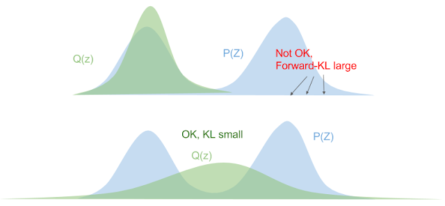
- Backward KL blows up if $q_{\phi}[x](z) \gg \Pr(z \mid x)$. This forces $q_{\phi}[x](Z)$ to "squeeze underneath" the true distribution. This is also called "mode-seeking" behaviour.


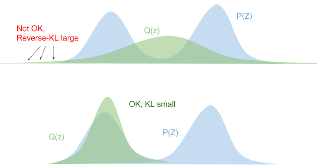
*Images from [Eric Jang: A Beginner's Guide to Variational Methods: Mean-Field Approximation](https://blog.evjang.com/2016/08/variational-bayes.html)*

Additionally, we must take practicality into consideration: taking the forward KL divergence would require us to sample from the true distribution $\Pr(Z \mid x),$ which is assumed to be intractable. On the other hand, we can get around this issue for the reverse case, which we'll demonstrate now.

### deriving the ELBO

Recall that our goal is to minimize the (reverse) KL divergence from our model $q_{\phi}[x](Z)$ to the "true" posterior distribution $\Pr(Z \mid x)$. By shuffling the $\log$s around a bit, we obtain the following:

$$D_{KL}(q_{\phi}[x](Z) || \Pr(Z \mid x)) = \log \Pr(x) - \mathbb{E}\left[\log \frac{\Pr(x, z)}{q_{\phi}[x](z)}\right]$$

(Try confirming this yourself!) Recall that we model $\Pr(x \mid z)$ by $p_{\theta}[z](x)$, which also lets us estimate $\Pr(x, z) \approx p_{\theta}[z](x) \pi(z),$ where in practice we set $\pi(Z)$ to be a standard multivariate Gaussian. All the expectations are taken w.r.t. our encoder $z \sim q_{\phi}[x](Z).$

Since $\log \Pr(x)$ (often called the "evidence") is constant w.r.t. our hyperparameters, minimizing the LHS is equivalent to maximizing the expected value term, which is called the **evidence based lower bound** (ELBO), since it provides a lower bound on the evidence (since KL divergence is nonnegative). (**Sidenote**: the fact that it's a lower bound can also be shown via Jensen's inequality.)

The ELBO term can also be expressed as

$$\mathbb{E}\left[ \log \frac{\Pr(x, z)}{q_{\phi}[x](z)} \right] \approx \mathbb{E}[\log p_{\theta}[z](x)] - D_{KL}(q_{\phi}[x](Z) || \pi(Z)),$$

where I've replaced $\Pr(x \mid z)$ with $p_{\theta}[z](x)$ and $\Pr(Z)$ with $\pi(Z)$. This now gives an explicit intuitive connection for how variational autoencoders connect to autoencoders!

- **Good reconstruction**: Maximizing the first term means that we want the original data to have a high likelihood after encoding and then decoding, which is essentially the probabilistic version of the $p_{\theta}(q_{\phi}(x)) \approx x$ intuition we had for autoencoders.
- **Regularizing the latent space**: Minimizing the KL divergence term is saying that we want the distribution $q_{\phi}[x](Z)$ to be "close" to the prior. This addresses the "discontinuous latent space" issue we had with deterministic autoencoders: now, we know that the latent space will be "tightly concentrated" around $\pi(Z),$ so by sampling from $\pi(Z)$ and decoding, we can generate images that look similar to ones from the true distribution $X$.

To recap, we've now come up with a well-formed objective: we seek to maximize the ELBO w.r.t. $\phi$ and $\theta$, which is equivalent to minimizing the reverse KL between $q_{\phi}[x](z)$ and the true posterior distribution. How do we actually do this?

## practical concerns

To actually fit a neural network or some other model to maximize the ELBO over the parameters $\phi$, we want to run gradient ascent on it (or equivalently gradient descent on its negation). Let's use the above decomposition into the "reconstruction likelihood" $\mathbb{E}[\log p_{\theta}[z](x)]$ and the "regularization term" $-D_{KL}(q_{\phi}[x](Z)||\Pr(Z))$.

### the reconstruction loss and the reparameterization trick

We can estimate the reconstruction loss using a simple Monte Carlo estimate, i.e. approximating the expectation by a sample mean. In practice, for each datapoint $x$, we simply "sample" a single $z$ to estimate this loss, though of course you could use draw more samples to trade efficiency for higher accuracy.

But this raises another issue: how do we differentiate through the sampling procedure? This isn't well-defined. Instead, we draw some independent standard multivariate normal noise $\varepsilon \in \mathbb{R}^{|\text{latent}|}$ and obtain $z$ by the **reparameterization** $z_{\ell} = \mu_{\ell} + \sigma_{\ell} \cdot \varepsilon_{\ell}$ for each dimension $\ell$ of the latent space. This is now clearly differentiable w.r.t. $\mu$ and $\sigma$.

Note that the original VAE paper goes into much deeper detail and generality regarding efficient gradient estimation. They also discuss what this reparameterization looks like for other distribution families.

- **Exercise**: consider distribution families whose parameters obey location-scale transformations. Can we reparameterize them in the same way as we did above?

### solving for the regularization term

We can often express the regularization term in a closed form. For example, Appendix B of the VAE paper presents the expression when $\pi(Z)$ is standard multivariate Gaussian and $q_{\phi}[x](Z)$ is also modelled as a isotropic multivariate Gaussian. (Though simple, this is a commonly used model in practice.) Then we can express

$$- 2 D_{KL}(q_{\phi}[x](z) || \Pr(Z)) = |\text{latent}| + \sum_{\ell=1}^{|\text{latent}|} \log \sigma_{\ell}^{2} - \|\mu\|_{2}^{2} - \|\sigma\|_{2}^{2},$$

where $(\mu, \sigma) = \tilde q_{\theta}[x] \in \Omega = \mathbb{R}^{|\text{latent}|} \times \mathbb{R}^{|\text{latent}|}$ as discussed earlier. As long as $\tilde q_{\phi}$ is differentiable w.r.t. $\phi,$ as is the case for any implementation we care about, then so is this objective, as desired.

Note that choosing an $\mathcal{F}_{Z}$ that assumes the elements of $Z$ are independent, as we do here, is called **mean-field** variational inference; not as scary as it might sound. One benefit of this assumption is that we can use fast algorithms that optimize over one element at a time, such as coordinate ascent; see [Princeton lecture notes from Professor David Blei](https://www.cs.princeton.edu/courses/archive/fall11/cos597C/lectures/variational-inference-i.pdf).

### finalizing the objective

Now we can differentiate both components of the ELBO objective w.r.t. $\phi$ and $\theta$, so we're all set to get implementing! For completeness, the final expression for the ELBO for our motivating example is given as

$$
\begin{gather*}
\text{ELBO} = \mathbb{E}\left[ \log \frac{\Pr(x, z)}{q_{\phi}[x](z)} \right] \approx \underbrace{\mathbb{E}[\log p_{\theta}[z](x)]}_{\text{reconstruction}} \underbrace{- D_{KL}(q_{\phi}[x](Z) || \pi(Z))}_{\text{regularization}} \\
= \left[ \sum_{i=1}^{|\text{input}|} x_{i} \log y_{i} + (1-x_{i}) \log (1-y_{i}) \right] + \left[ \frac{1}{2} \sum_{\ell=1}^{|\text{latent}|}(1 + \log \sigma_{\ell}^{2} - \mu_{\ell}^{2} - \sigma_{\ell}^{2}) \right] \\
\text{where} \quad z_{\ell} = \mu_{\ell}+ \sigma_{\ell} \varepsilon_{\ell}, \quad \varepsilon_{\ell} \sim \mathcal{N}(0, 1) \quad \forall \ell = 1, \dots, |\text{latent}| \\
\mu, \sigma = \tilde q_{\phi}[x], \quad y = \tilde p_{\theta}[z]
\end{gather*}
$$

Phew! It looks intimidating, but the code is really just a couple lines. I link to my Jax implementation in the conclusion.

To derive the first term, $\log p_{\theta}[z](x)$, remember that $p_{\theta}$ maps from $\mathcal{Z}$ to *distributions* over $\mathcal{X}$, not deterministically to $\mathcal{X}$! Here it's just a coincidence that the parameter space coincides with the variable space since we chose $\mathcal{F}_{X}$ to be independent Bernoulli trials. In this case, the output of our decoder should be $y \in [0, 1]^{|\text{input}|}$, where each element describes the probability of that pixel being white. This can be easily done by applying an elementwise sigmoid as the final layer. Then we have

$$\log p_{\theta}[z](x) = \sum_{i=1}^{|\text{input}|} x_{i} \log y_{i} + (1-x_{i}) \log (1-y_{i}).$$

Similarly, if our data were Gaussian, the output of the decoder should be $\mu, \sigma \in \mathbb{R}^{|\text{input}|}$ (assuming the elements of $X$ are conditionally independent given $Z$), and we could calculate the log-likelihood as follows, where I multiply by $-2$ for brevity, and also use an elementwise division by $\sigma$ in the last term:

$$-2 \log p_{\theta}[z](x) = |\text{input}| \log 2 \pi + \sum_{i=1}^{|\text{input}|} \log \sigma_{i}^{2} + \left\| \frac{x - \mu}{\sigma} \right\|_{2}^{2}.$$

This gives us all the tools we need to optimize over $\phi, \theta$ to maximize the ELBO and minimize $D_{KL}(q_{\phi}[x](Z) || \Pr(Z \mid x))$.

## conclusion

I hope you enjoyed reading! [Here's](https://colab.research.google.com/drive/1v0UiRwUiBi4IoZKXXnwZwHpVDsUIoeg0?usp=sharing) an implementation I wrote in pure Jax that also contains some fun visualizations from their original paper. I like Jax because of the pure functional programming style that makes the dependencies and types of each function very clear. If you're interested, play around with the optimization hyperparameters and see if you can get prettier results; my learned MNIST manifold doesn't look quite as clean as the paper's Figure 4.

## sources

[Auto-Encoding Variational Bayes - Kingma and Welling](https://arxiv.org/abs/1312.6114)
- The original VAE paper. I found the notation somewhat frustrating but it's quite well written and also goes into more detail about 1) including $\phi, \theta$ in the variational optimization and 2) about how VAEs generalize beyond the assumptions made here.

[Eric Jang: A Beginner's Guide to Variational Methods: Mean-Field Approximation](https://blog.evjang.com/2016/08/variational-bayes.html)
- Helpful visualization of forward vs reverse KL divergence.

[From Autoencoder to Beta-VAE | Lil'Log](https://lilianweng.github.io/posts/2018-08-12-vae/)
- Goes further into depth on related architectures including denoising / sparse / contractive autoencoders and later research including $\beta$-VAEs, vector quantized VAEs, and temporal difference VAEs.

[Princeton lecture notes from Professor David Blei](https://www.cs.princeton.edu/courses/archive/fall11/cos597C/lectures/variational-inference-i.pdf)
- Very in-depth and focuses on the optimization algorithms, which I've waved away in this post under the umbrella of "gradient ascent".
- Walks through a concrete example of a simple distribution whose posterior is hard to calculate: a mixture of Gaussians where the centroids are drawn from a Gaussian.
- Describes an improvement when $\mathcal{F}_{Z}$ is such that the distribution of each element, conditional on the others and on $x$, belongs to an exponential family.