Progressive Growing of GANs for Improved Quality, Stability, and Variation
===

- ref:
- [Sarah Wolf: ProGAN: How NVIDIA Generated Images of Unprecedented Quality](https://towardsdatascience.com/progan-how-nvidia-generated-images-of-unprecedented-quality-51c98ec2cbd2)
- [AIHelsinki 15.2.2018: Tero Karras, NVIDIA](https://www.youtube.com/watch?v=ReZiqCybQPA)


> ProGAN uses nearest neighbors for upscaling and average pooling for downscaling.


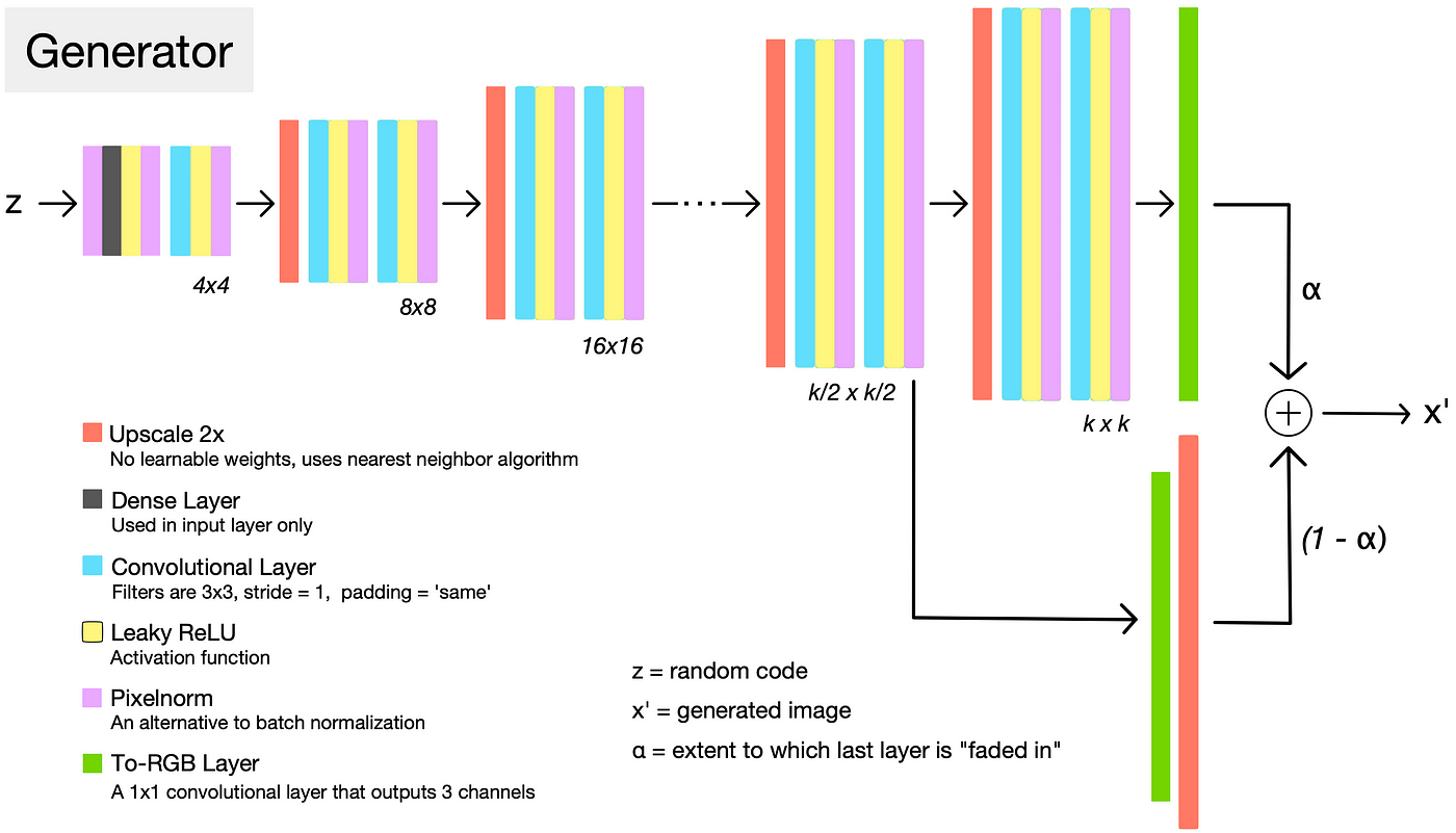
> A detailed view of the generator architecture, when it has “grown” to resolution k. Each set of layers doubles the resolution size with a nearest neighbor upscaling operation followed by two convolutions.

**Fading in**

> To stabilize training, the most recently added layer is “faded in”. This process is controlled by α, a number between 0 and 1 that is linearly increased over many training iterations until the new layer is fully in place.

**Pixel Normalization**


> Instead of using batch normalization, as is commonly done, the authors used pixel normalization.

> It normalizes the feature vector in each pixel to unit length, and is applied after the convolutional layers in the generator

> This is done to prevent signal magnitudes from spiraling out of control during training.

> The values of each pixel (x, y) across C channels are normalized to a fixed length.

**Discriminator**


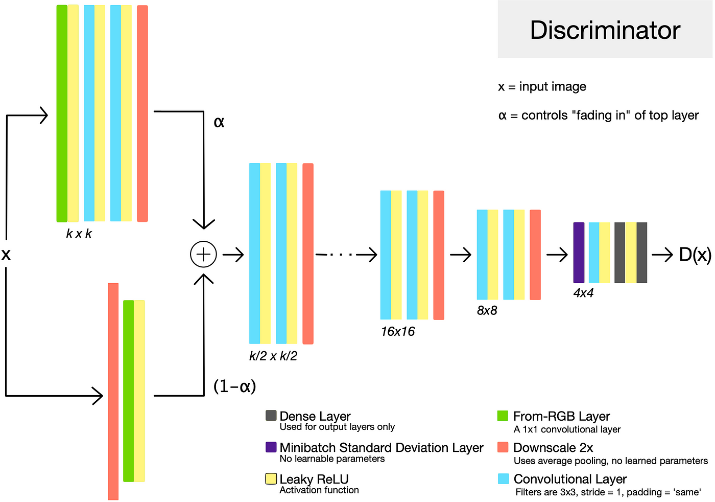
**Minibatch Standard Deviation**

> In general, GANs tend to produce samples with less variation than that found in the training set.

> One approach to combat this is to have the discriminator compute statistics across the batch, and use this information to help distinguish the “real” training data batches from the “fake” generated batches.

> This encourages the generator to produce more variety, such that statistics computed across a generated batch more closely resemble those from a training data batch.

> This layer has no trainable parameters. It computes the standard deviations of the feature map pixels across the batch, and appends them as an extra channel.

**Equalized Learning Rate**


> The authors found that to ensure healthy competition between the generator and discriminator, it is essential that layers learn at a similar speed.

> To achieve this equalized learning rate, they scale the weights of a layer according to how many weights that layer has.

> For example, before performing a convolution with f filters of size [k, k, c], we would scale the weights of those filters as shown above.

> Due to this intervention, no fancy tricks are needed for weight initialization — simply initializing weights with a standard normal distribution works fine.

> [color=#1efcc8][name=Yu Kai Huang] 為何這樣會 Equalized?

**Loss Function**


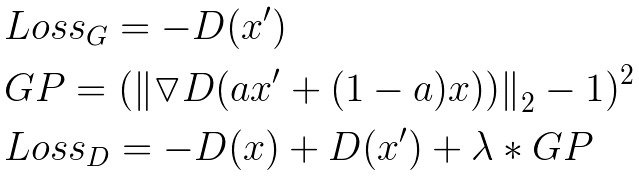
> The authors say that the choice of loss function is orthogonal to their contribution — meaning that none of the above improvements rely on a specific loss function.

> they used the improved Wasserstein loss function, also known as WGAN-GP.

> It is one of the fancier common loss functions, and has been shown to stabilize training and improve the odds of convergence.

> WGAN-GP loss function expects D(x) and D(x’) to be unbounded real-valued numbers. In other words, the output of the discriminator is not expected to be a value between 0 and 1. This is slightly different than the traditional GAN formulation, which views the output of the discriminator as a probability.

> x’: generated image
> x: an image from the training set
> D: the discriminator
> GP: gradient penalty that helps stabilize training.
> a: term in the gradient penalty refers to a tensor of random numbers between 0 and 1, chosen uniformly at random.
> λ = 10.

--

> starting from easier low-resolution images, and add new layers that introduce higher-resolution details as the training progresses

> When new layers are added to the networks, we fade them in smoothly

- inception score: 8.80 in unsupervised CIFAR10
- new metric
- subtle modification to the initialization of network
- 2–6 times faster to get comparable result quality
- CelebA-HQ

Related
---

- Wang et al. (2017)
- use multiple discriminators that operate on different spatial resolutions.

Main
---

- PROGRESSIVE GROWING OF GANS
- When new layers are added to the networks, we fade them in smoothly
- transition: weight α increases linearly from 0 to 1
- INCREASING VARIATION USING MINIBATCH STANDARD DEVIATION
- 對 feature 做了一些轉換 -> 目的: orthogonalize the feature vectors in a minibatc?
- v.s. minibatch discrimination (Salimans et al., 2016)
- equalized learning rate: more balanced learning speed for different layers
- through careful weight initialization
- wi = wi / c (He’s initializer) (He et al., 2015)
- training configuration: (a)-(h)
- CelebA-HQ
- 30000 images
- 1024 × 1024 resolution

Metric
---

- SWD (sliced Wasserstein distance)
- MS-SSIM
- inception score

Loss
---

- WGAN-GP loss (improved Wasserstein loss)
- L' = L + e_drift*E(D(x)^2)
- LSGAN loss (least-squares loss)
- v.s. WGAN-GP loss => authors pefer WGAN-GP loss!
- a less stable loss function than WGAN-GP
- lose some of the variation towards the end of long runs

Future
---

> Tero Karras: Image editing



> Tero Karras: Digital humans


> [color=#1efcc8][name=Yu Kai Huang] DVD-GAN? https://arxiv.org/abs/1907.06571

> Tero Karras: Content creation


Ref
---

- inception score (Salimans et al., 2016)
- multi-scale structural similarity (MS-SSIM) (Odena et al., 2017; Wang et al., 2003)
- conceptual similarity to recent work by Chen & Koltun (2017)