# Disribution

### What is Distribution?

A probability distribution is a statistical function that describes all the possible values and probabilities for a random variable within a given range. This range will be bound by the minimum and maximum possible values, but where the possible value would be plotted on the probability distribution will be determined by a number of factors. The mean (average), standard deviation, skewness, and kurtosis of the distribution are among these factors.

#### Types of Distribution
1. Discrete Probability Distributions

A discrete distribution is one in which the data can only take on certain values
1. Binomial Distrobution
2. Poisson Distribution
3. Bernoulli Distribution
2. Continuous Probability Distributions

A continuous distribution is one in which data can take on any value within a specified range
1. Normal Distribution
2. t- Distribution
3. Uniform Distribution
4. Exponential Distribution
5. Chi-square Distribution
6. F- Distribution

### Why do we need distribution?
Sampling distributions are important for statistics because we need to collect the sample and estimate the parameters of the population distribution. Hence distribution is necessary to make inferences about the overall population.

### How to apply test of hypothesis on data?
Hypothesis Testing is a type of statistical analysis in which you put your assumptions about a population parameter to the test. It is used to estimate the relationship between 2 statistical variables.

<br>**Null Hypothesis and Alternate Hypothesis**
The Null Hypothesis is the assumption that the event will not occur. A null hypothesis has no bearing on the study's outcome unless it is rejected.

H0 is the symbol for it, and it is pronounced H-naught.

The Alternate Hypothesis is the logical opposite of the null hypothesis. The acceptance of the alternative hypothesis follows the rejection of the null hypothesis. H1 is the symbol for it.

### Steps of Hypothesis Testing

<br>**Step 1**: **Specify Your Null and Alternate Hypotheses**
It is critical to rephrase your original research hypothesis (the prediction that you wish to study) as a null (Ho) and alternative (Ha) hypothesis so that you can test it quantitatively. Your first hypothesis, which predicts a link between variables, is generally your alternate hypothesis. The null hypothesis predicts no link between the variables of interest.

**Step 2**: **Gather Data**
For a statistical test to be legitimate, sampling and data collection must be done in a way that is meant to test your hypothesis. You cannot draw statistical conclusions about the population you are interested in if your data is not representative.

**Step 3**: **Conduct a Statistical Test**
Other statistical tests are available, but they all compare within-group variance (how to spread out the data inside a category) against between-group variance (how different the categories are from one another). If the between-group variation is big enough that there is little or no overlap between groups, your statistical test will display a low p-value to represent this. This suggests that the disparities between these groups are unlikely to have occurred by accident. Alternatively, if there is a large within-group variance and a low between-group variance, your statistical test will show a high p-value. Any difference you find across groups is most likely attributable to chance. The variety of variables and the level of measurement of your obtained data will influence your statistical test selection.

**Step 4**: **Determine Rejection Of Your Null Hypothesis**
Your statistical test results must determine whether your null hypothesis should be rejected or not. In most circumstances, you will base your judgment on the p-value provided by the statistical test. In most circumstances, your preset level of significance for rejecting the null hypothesis will be 0.05 - that is, when there is less than a 5% likelihood that these data would be seen if the null hypothesis were true. In other circumstances, researchers use a lower level of significance, such as 0.01 (1%). This reduces the possibility of wrongly rejecting the null hypothesis.

**Step 5**: **Present Your Results**
The findings of hypothesis testing will be discussed in the results and discussion portions of your research paper, dissertation, or thesis. You should include a concise overview of the data and a summary of the findings of your statistical test in the results section. You can talk about whether your results confirmed your initial hypothesis or not in the conversation. Rejecting or failing to reject the null hypothesis is a formal term used in hypothesis testing. This is likely a must for your statistics assignments.

### Types of Hypothesis Testing
<br>**Z Test**
To determine whether a discovery or relationship is statistically significant, hypothesis testing uses a z-test. It usually checks to see if two means are the same (the null hypothesis). Only when the population standard deviation is known and the sample size is 30 data points or more, can a z-test be applied.

**T Test**
A statistical test called a t-test is employed to compare the means of two groups. To determine whether two groups differ or if a procedure or treatment affects the population of interest, it is frequently used in hypothesis testing.

**Chi-Square**
You utilize a Chi-square test for hypothesis testing concerning whether your data is as predicted. To determine if the expected and observed results are well-fitted, the Chi-square test analyzes the differences between categorical variables from a random sample. The test's fundamental premise is that the observed values in your data should be compared to the predicted values that would be present if the null hypothesis were true.

### Hypothesis Testing and Confidence Intervals
Both confidence intervals and hypothesis tests are inferential techniques that depend on approximating the sample distribution. Data from a sample is used to estimate a population parameter using confidence intervals. Data from a sample is used in hypothesis testing to examine a given hypothesis. We must have a postulated parameter to conduct hypothesis testing.

A variety of feasible population parameter estimates are included in confidence ranges. In this lesson, we created just two-tailed confidence intervals. There is a direct connection between these two-tail confidence intervals and these two-tail hypothesis tests. The results of a two-tailed hypothesis test and two-tailed confidence intervals typically provide the same results. In other words, a hypothesis test at the 0.05 level will virtually always fail to reject the null hypothesis if the 95% confidence interval contains the predicted value. A hypothesis test at the 0.05 level will nearly certainly reject the null hypothesis if the 95% confidence interval does not include the hypothesized parameter.

#### Simple and Composite Hypothesis Testing
Depending on the population distribution, you can classify the statistical hypothesis into two types.

1. **Simple Hypothesis**: A simple hypothesis specifies an exact value for the parameter.

2. **Composite Hypothesis**: A composite hypothesis specifies a range of values.

### **Normal Distribution**

A normal distribution is a type of continuous probability distribution in which most data points cluster toward the middle of the range, while the rest taper off symmetrically toward either extreme. The middle of the range is also known as the mean of the distribution.

The normal distribution is also known as a Gaussian distribution or probability bell curve. It is symmetric about the mean and indicates that values near the mean occur more frequently than the values that are farther away from the mean.

<br>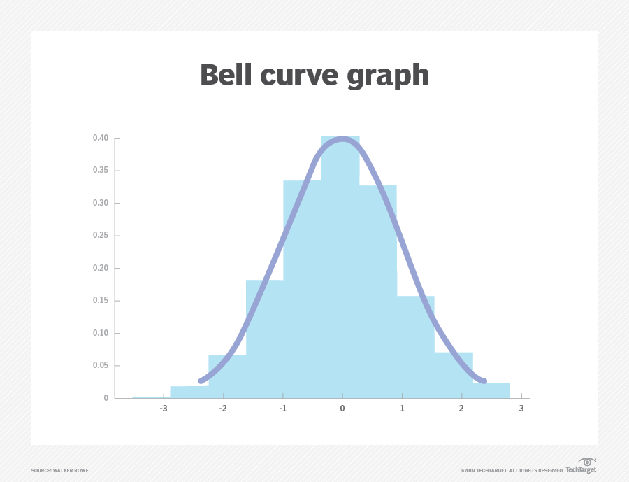

### Importance of normal distribution
1. It describes the distribution of values for many natural phenomena in a wide range of areas, including biology, physical science, mathematics, finance and economics. It can also represent these random variables accurately.

2. It is used to approximate other type of probability distribution like such as `binomial`, `Poisson distribution`, etc.

> Normal approximation of binomial distribution
<br>

3. Normal distribution is the key idea behind the central limit theorem, or CLT, which states that averages calculated from independent, identically distributed random variables have approximately normal distributions. This is true regardless of the type of distribution from which the variables are sampled, as long as it has finite variance.

#### Example of normal distribution

1. An automobile company is looking for fuel additives that might increase gas mileage. Without additives, their cars are known to average `25 mpg (miles per gallons)` with a standard deviation of `2.4mpg` on a road trip from London to Edinburgh. The company now asks whether a particular new additive increases this value. In a study, thirty cars are sent on a road trip from London to Edinburgh. Suppose it turns out that the thirty cars averaged `x = 25.5 mpg` with the additive. Can we conclude from this result that the additive is effective?

##### Solution

We are asked to show if the new additive increases the mean miles per gallon. The current mean `μ = 25` so the null hypothesis will be that nothing changes. The alternative hypothesis will be that `μ > 25` because this is what we have been asked to test.
<br> H~0~:μ = 25.
<br> H~1~:μ > 25.
<br> Now we need to calculate the test statistic. We start with the assumption the normal distribution is still valid. This is because the null hypothesis states there is no change in `μ`. Thus, as the value `σ = 2.4 mpg` is known, we perform a hypothesis test with the standard normal distribution. So the test statistic will be a `z` score. We compute the `z` score using the formula
<br> `z=(¯x − μ)/(σ/√n)`
<br>So
<br>`z = (¯x − 25)/(2.4/√30) = 1.14`
We are using a `5%` significance level and a (right-sided) one-tailed test, so `α = 0.05` so from the tables we obtain z~1−α~ = 1.645 is our test statistic. As `1.14 < 1.645`, the test statistic is not in the critical region so we cannot reject H~0~. Thus, the observed sample mean `¯x = 25.5` is consistent with the hypothesis H~0~:μ = 25 on a `5%` significance level.
<br>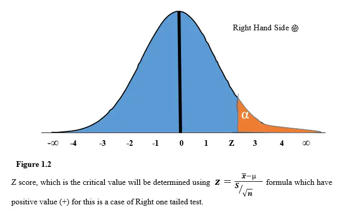
<br>If calculated z > z~α~ i.e we are in critical region so we reject H~0~