# Hashmap Implementation
---
## Check if given element exists in Q queries
Given an array of size N and Q queries. In each query, an element is given. We have to check whether that element exists or not in the given array.
**Example**
A [ ] = {`2, 4, 11, 15 , 6, 8, 14, 9`}
`4 Queries`
`K = 4` (return true)
`K = 10` (return false)
`K = 17` (return false)
`K = 14` (return true)
:::warning
Please take some time to think about the solution approach on your own before reading further.....
:::
#### Brute Force Approach
For every query, loop through the given array to check the presence.
Time Complexity - **O(N * Q)**
Space Complexity - **O(1)**
#### Observation
We can create an array to mark the presence of an element against that particular index.
A [ ] = {`2, 4, 11, 15 , 6, 8, 14, 9`}
For example we can mark presence of
2 at index 2
4 at index 4 and so on....
To execute that, we'll need to have indices till 15(max of Array).
The array size needed is 16.
Let's call that array as - DAT (Direct Access Table)
int dat[16] = {0}; //initally assuming an element is not present
| 0 | 1 | 2 | 3 | 4 | 5 | 6 | 7 | 8 | 9 | 10 | 11 | 12 | 13 | 14 | 15 |
| -------- | -------- | -------- | -------- | -------- | -------- | -------- | -------- | -------- | -------- | -------- | -------- | -------- | -------- | -------- | -------- |
| 0 | 0 | 0 | 0 | 0 | 0 | 0 | 0 | 0 | 0 | 0 | 0 | 0 | 0 | 0 | 0 |
Let's mark the presence.
```cpp
for(int i = 0; i < N; i++) {
dat[A[i]] = 1;
}
```
Below is how that array looks like -
| 0 | 1 | 2 | 3 | 4 | 5 | 6 | 7 | 8 | 9 | 10 | 11 | 12 | 13 | 14 | 15 |
| -------- | -------- | -------- | -------- | -------- | -------- | -------- | -------- | -------- | -------- | -------- | -------- | -------- | -------- | -------- | -------- |
| 0 | 0 | 1 | 0 | 1 | 0 | 1 | 0 | 1 | 1 | 0 | 1 | 0 | 0 | 1 | 1 |
#### Advantage of using DAT
1. Time Complexity of Insertion - `O(1)`
2. Time Complexity of Deletion - `O(1)`
3. Time Complexity of Search - `O(1)`
#### Issues with such a representation
**1. Wastage of Space**
* Say array is `A[] = {23, 60, 37, 90}`; now just to store presence of 4 elements, we'll have to construct an array of `size 91`.
**2. Inability to create big Arrays**
* If values in array are as big as $10^{15}$, then we will not be able to create this big array. At max array size possible is 10^6^(around)
**3. Storing values other than positive Integers**
* We'll have to make some adjustments to store negative numbers or characters. (It'll be possible but needs some work-around)
---
### Overcome Issues while retaining Advantages
Let's say we have restriction of creating only array of size 10.
Given Array -
A [ ] = {`21, 42, 37, 45 , 99, 30`}
**How can we do so ?**
In array of size 10, we'll have indices from 0 to 9. How can we map all the values within this range ?
**Basically, we can take a mod with 10.**
21 % 10 = 1 (presence of 21 can be marked at index 1)
42 % 10 = 2 (presence of 42 can be marked at index 2)
37 % 10 = 7 (presence of 37 can be marked at index 7)
45 % 10 = 5 (presence of 45 can be marked at index 5)
99 % 10 = 9 (presence of 99 can be marked at index 9)
30 % 10 = 0 (presence of 30 can be marked at index 0)
| 0 | 1 | 2 | 3 | 4 | 5 | 6 | 7 | 8 | 9 |
| -------- | -------- | -------- | -------- | -------- | -------- | -------- | -------- | -------- | -------- |
| 30 | 21 | 42 | 0 | 0 | 45 | 0 | 37 | 0 | 99 |
#### What Have We Done ?
* We have basically done Hashing. Hashing is a process where we pass our data through the Hash Funtion which gives us the hash value(index) to map our data to.
* In this case, the hash function used is **MOD**. This is the simplest hash function. Usually, more complex hash functions are used.
* The DAT that we created is known as **Hash Table** in terms of Hashing.
#### Issue with Hashing ?
**COLLISION!**
Say given array is as follows -
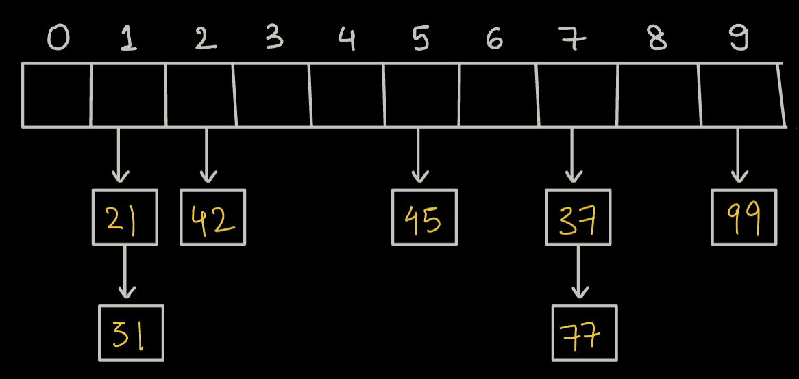
A [ ] = {21, 42, 37, 45, 77, 99, 31}
Here, 21 & 31 will map to the same index => 1
37 & 77 map to same index => 7
**Can we completely avoid collision ?**
`Not Really!`
No matter how good a hash function is, we can't avoid collision!
**Why ?**
We are trying to map big values to a smaller range, collisions are bound to happen.
Moreover, this can be explained using `Pigeon Hole Principle!`
**Example -**
Say we have 11 pigeons and we have only 8 holes to keep them. Now, provided holes are less, atleast 2 pigeons need to fit in a single hole.
But, we can find some resolutions to collision.
---
### Collision Resolution Techniques
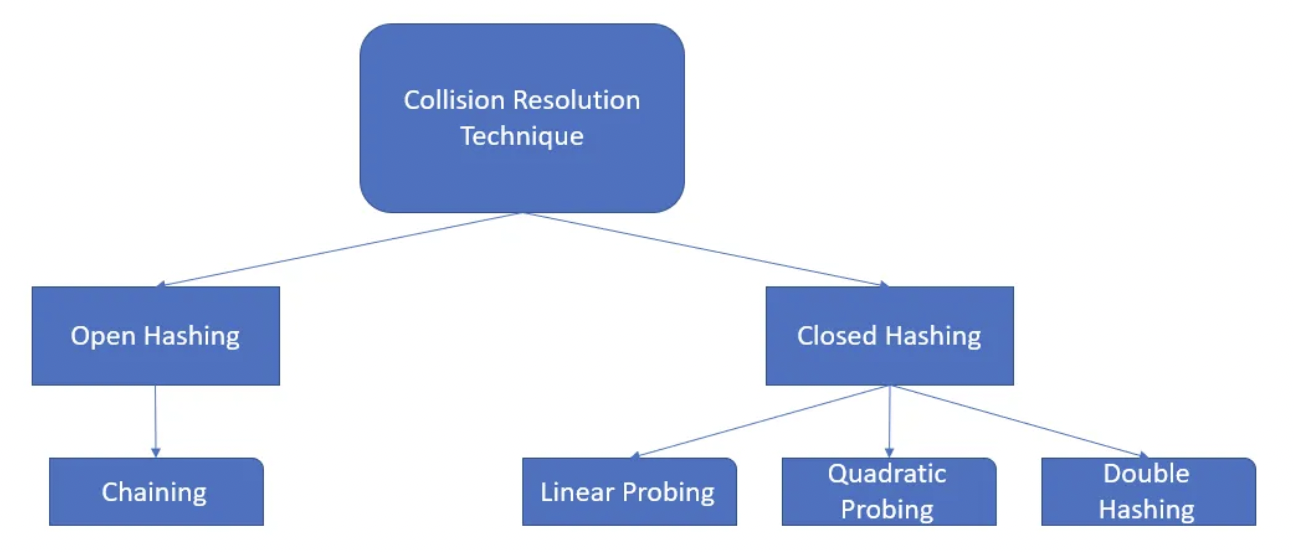
>From Interview Perspective, Open Hashing is Important hence, we'll dive into that.
---
### Chaining
Let's take the above problem where collision happened!
A [ ] = {`21, 42, 37, 45, 77, 99, 31`}
Here, 21 & 31 will map to the same index => 1
37 & 77 map to same index => 7
**How can we resolve Collision here?**
We can somehow store both 21 & 31 at the same index.
Basically we can have a linked list at every index.
i.e, Array of Linked List
Every index shall have head node of Linked List.
**The above method is known as Chaining.**
* **Chaining** is a technique used in data structures, particularly hash tables, to resolve collisions. When multiple items hash to the same index, chaining stores them in a linked list or another data structure at that index.
**What will be the Time Complexity of Insertion ?**
* First we will pass the given element to Hash Function, which will return an index. Now, we will simply add that element to the Linked List at that index.
* If we insert at **tail** => `O(N)`
* If we insert at **head** => `O(1)`
Since order of Insertion doesn't matter to us, so we can **simply insert at head**.
**What will be the Time Complexity of Deletion and Searching ?**
* Time Complexity on average is always less than $\lambda$. $\lambda$ is known as lamda.
* Time Complexity in worst case is still O(N)
---
### What is lamda
There is a lamba($\lambda$) function which is nothing but a ratio of (number of elements inserted / size of the array).
**Example:**
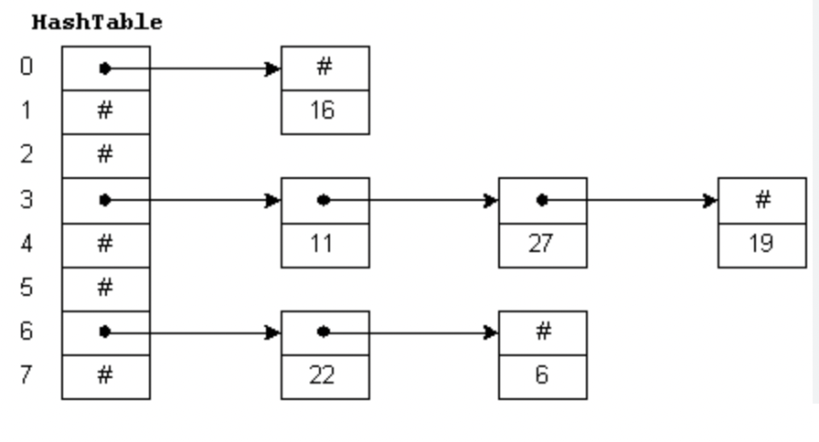
Table size(Array size) = 8
Inserted Elements = 6
$\lambda$ = $\frac{6}{8}$ = 0.75
Let's assume the predefined threshold is 0.7. The load factor is exceeding this value, so we will need to rehash the table.
**Rehashing:**
* Create a new hash table with double the size of the original hash table. In this case, the new size will be
* 8×2=16
* Redistribute the existing elements to their new positions in the larger hash table using a new hash function.
* The load factor is now recalculated for the new hash table:
*
$\lambda$ = $\frac{6}{16} = 0.375$ (within the threshold of 0.7)
---
### Code Implementation
#### Declaring the HashMap Class
Let's go through the code implementation of a hashmap:
* The HashMap class is defined with generic types `K` and `V` for keys and values.
* The inner class `HMNode` represents a node containing a key-value pair.
* `buckets` is an array of ArrayLists to store key-value pairs.
* `size` keeps track of the number of key-value pairs in the hashmap.
* The `initbuckets()` method initializes the array of buckets with a default size of 4.
```java
import java.util.ArrayList;
class HashMap < K, V > {
private class HMNode {
K key;
V value;
public HMNode(K key, V value) {
this.key = key;
this.value = value;
}
}
private ArrayList < HMNode > [] buckets;
private int size; // number of key-value pairs
public HashMap() {
initbuckets();
size = 0;
}
private void initbuckets() {
buckets = new ArrayList[4];
for (int i = 0; i < 4; i++) {
buckets[i] = new ArrayList < > ();
}
}
```
#### Put Method
* The `put` method adds a key-value pair to the hashmap.
* It calculates the bucket index (`bi`) using the `hash` method and finds the data index within the bucket using `getIndexWithinBucket`.
* If the key is found in the bucket, it updates the value. Otherwise, it inserts a new node.
* After inserting, it checks the load factor (`lambda`) and triggers rehashing if the load factor exceeds 2.0.
```java
public void put(K key, V value) {
int bi = hash(key);
int di = getIndexWithinBucket(key, bi);
if (di != -1) {
// Key found, update the value
buckets[bi].get(di).value = value;
} else {
// Key not found, insert new key-value pair
HMNode newNode = new HMNode(key, value);
buckets[bi].add(newNode);
size++;
// Check for rehashing
double lambda = size * 1.0 / buckets.length;
if (lambda > 2.0) {
rehash();
}
}
}
```
#### Hash Method
* The `hash` method calculates the bucket index using the hash code of the key and takes the modulus to ensure it stays within the array size.
```java
private int hash(K key) {
int hc = key.hashCode();
int bi = Math.abs(hc) % buckets.length;
return bi;
}
```
#### Get Index within Bucket
* The `getIndexWithinBucket` method searches for the data index (`di`) of a key within a specific bucket. It returns -1 if the key is not found
```java
private int getIndexWithinBucket(K key, int bi) {
int di = 0;
for (HMNode node: buckets[bi]) {
if (node.key.equals(key)) {
return di; // Key found
}
di++;
}
return -1; // Key not found
}
```
#### Rehash Method
* The `rehash` method is called when the load factor exceeds 2.0.
* It creates a new array of buckets, initializes the size to 0, and iterates through the old buckets, reinserting each key-value pair into the new array.
*
```java
private void rehash() {
ArrayList < HMNode > [] oldBuckets = buckets;
initbuckets();
size = 0;
for (ArrayList < HMNode > bucket: oldBuckets) {
for (HMNode node: bucket) {
put(node.key, node.value);
}
}
}
```
#### Get Method
* The `get` method retrieves the value associated with a given key. It calculates the bucket index and searches within the bucket to find the key.
```java
public V get(K key) {
int bi = hash(key);
int di = getIndexWithinBucket(key, bi);
if (di != -1) {
return buckets[bi].get(di).value;
} else {
return null;
}
}
```
#### Contains Key Method
* The `containsKey` method checks if a given key exists in the hashmap by calculating the bucket index and checking the data index within the bucket.
```java
public boolean containsKey(K key) {
int bi = hash(key);
int di = getIndexWithinBucket(key, bi);
return di != -1;
}
```
#### Remove Method
* The `remove` method removes a key-value pair from the hashmap. If the key is found, it returns the value; otherwise, it returns null
```java
public V remove(K key) {
int bi = hash(key);
int di = getIndexWithinBucket(key, bi);
if (di != -1) {
// Key found, remove and return value
size--;
return buckets[bi].remove(di).value;
} else {
return null; // Key not found
}
}
```
#### Size Method
The `size` method returns the total number of key-value pairs in the hashmap.
```java
public int size() {
return size;
}
```
#### Key Set Method
* The `keyset` method returns an ArrayList containing all the keys in the hashmap by iterating through the buckets and nodes.
```java
public ArrayList < K > keyset() {
ArrayList < K > keys = new ArrayList < > ();
for (ArrayList < HMNode > bucket: buckets) {
for (HMNode node: bucket) {
keys.add(node.key);
}
}
return keys;
}
}
```
---
### Question
What is the time complexity of the brute-force approach for checking the existence of an element in the array for Q queries?
**Choices**
- [ ] O(N)
- [ ] O(Q)
- [x] O(N * Q)
- [ ] O(1)
---
### Question
What advantage does the Direct Access Table (DAT) provide in terms of time complexity for insertion, deletion, and search operations?
**Choices**
- [x] O(1) for all operations
- [ ] O(N) for all operations
- [ ] O(1) for insertion and deletion, O(N) for search
- [ ] O(N) for insertion and deletion, O(1) for search
---
### Question
What is the purpose of the load factor (lambda) in a hashmap?
**Choices**
- [ ] It represents the number of elements in the hashmap.
- [ ] It is used to calculate the hash code of a key.
- [x] It determines when to trigger rehashing.
- [ ] It controls the size of the hashmap.
---
### Question
What does the rehashing process involve in a hashmap?
**Choices**
- [ ] Reducing the size of the hashmap
- [x] Creating a new hash table with double the size and redistributing elements
- [ ] Deleting all elements from the hashmap
- [ ] Removing collision resolution techniques
 Sign in with Wallet
Connect another wallet
Sign in with Wallet
Connect another wallet