---
date: 1 February 2020
category: CMSC57
description: Computer science often work with large amounts of data. This can be observed in the fields of machine learning, data science, and computer graphics. Thankfully mathematical structures representing large amounts of data has been an established field in mathematics long before computers. In this topic we will study how these structures work, and how these structures are represented. Even though these representations are beyond human imagination.
---

# Introduction to Linear Algebra

## Matrices and Matrix Operations

A matrix is a **rectangular collection** of numbers. The matrix below called matrix $A$ is a $2 \times 3$ matrix. Meaning it has 2 rows and 3 columns.

$$
A=\begin{bmatrix}
4&2&-3 \\
11&\pi & 12
\end{bmatrix}
$$

The matrix below called $B$ is a $4 \times 1$ matrix meaning it has $4$ rows and $1$ column.

$$
B=\begin{bmatrix}
1\\
34\\
-12\\
0
\end{bmatrix}
$$
Matrices are important mathematical structures to computer science because they are used to represent a collection of numbers. A png image for example is defined by arranging the value of each pixel's values in a matrix. A grayscale image like the one below is defined using pixel brightness values.

$$
A=\begin{bmatrix}
0.1&0.9&0.3 \\
0.4&0.5&0.6 \\
0.7&0.7&0.9
\end{bmatrix}
$$


An **element** of a matrix is denoted by $a_{rc}$ which corresponds the element of matrix $a$ in the $r^{th}$ row and $c^{th}$ column. Using the examples above, The element,
$$
a_{23}=12
$$

$$
A=\begin{bmatrix}
a_{11}&a_{12}&a_{13} \\
a_{21}&a_{22}&a_{23}
\end{bmatrix}
$$

Matrices are also generally used to represent **systems of linear equations** for example:

$$
\begin{aligned}
4x + 2y =12 \\
3x - 2y = 8
\end{aligned}
$$

Is represented using a matrix:

$$
\begin{bmatrix}
4&2\\
3&-28
\end{bmatrix}
\begin{bmatrix}
x\\
y
\end{bmatrix}=
\begin{bmatrix}
12\\
8
\end{bmatrix}
$$

> how this works will be explained later

### Matrix Arithmetic

#### Matrix Addition

Matrices can be added and multiplied to scalar values (non matrices), and other matrices.

Matrix addition is trivial, let $A$ and $B$ be $m\times n$ matrices:

$$
A+B=\begin{bmatrix}
a_{11}+b_{11}&a_{12}+b_{12}&\dots&a_{1n}+b_{1n} \\
a_{21}+b_{21}&a_{22}+b_{22}&\dots&a_{2n}+b_{2n} \\
\vdots&\vdots&\ddots&\vdots \\
a_{m1}+b_{m1}&a_{m2}+b_{m2}&\dots&a_{mn}+b_{mn}
\end{bmatrix}\\
$$

To get each element$(A+B)_{ij}$, you simply **add the corresponding elements**, $a_{11}+b_{11}$. Because of this you cannot add two matrices if their sizes differ.

Scalar plus matrix works similarly

$$
A+x=\begin{bmatrix}
a_{11}+x&a_{12}+x&\dots&a_{1n}+x \\
a_{21}+x&a_{22}+x&\dots&a_{2n}+x \\
\vdots&\vdots&\ddots&\vdots \\
a_{m1}+x&a_{m2}+x&\dots&a_{mn}+x
\end{bmatrix}\\
$$

#### Matrix Multiplication

**Matrix times matrix** multiplication works differently, let say $A$ is an $m \times k$ matrix and $B$ is a $k \times n$ matrix. Their **cross product** $C=A \times B$ defined to be the matrix with each element:

$$
c_{ij}=a_{i1}b_{1j}+a_{i2}b_{2j}+\cdots+a_{ik}b_{kj}
$$

For example

$$
A\times B=\begin{bmatrix}
a_{11}&a_{12}&\dots&a_{1n} \\
a_{21}&a_{22}&\dots&a_{2n} \\
\vdots&\vdots& &\vdots \\
a_{i1}&a_{i2}&\cdots&a_{in}\\
\vdots&\vdots& &\vdots \\
a_{m1}&a_{m2}&\dots&a_{mn}
\end{bmatrix} \times
\begin{bmatrix}
b_{11}&b_{12}&\dots&b_{1j}&\dots&b_{1n} \\
b_{21}&b_{22}&\dots&b_{1j}&\dots&b_{2n} \\
\vdots&\vdots&\ &\vdots& &\vdots \\
b_{m1}&b_{m2}&\dots&b_{1j}&\dots&b_{mn}
\end{bmatrix}=
\begin{bmatrix}
c_{11}&c_{12}&\dots&c_{1n} \\
c_{21}&c_{22}&\dots&c_{2n} \\
\vdots&\vdots&c_{ij}&\vdots \\
c_{m1}&c_{m2}&\dots&c_{mn}
\end{bmatrix}\\
$$

**Scalar times matrix** multiplication works similar to scalar plus matrix addition:
$$
Ax=\begin{bmatrix}
a_{11}x&a_{12}x&\dots&a_{1n}x \\
a_{21}x&a_{22}x&\dots&a_{2n}x \\
\vdots&\vdots&\ddots&\vdots \\
a_{m1}x&a_{m2}x&\dots&a_{mn}x
\end{bmatrix}\\
$$

### Special Matrices

#### Identity Matrix

The **identity matrix** $I_n$ of order $n$ is a special $n \times n$ (square) matrix such that its elements $\iota_{ij}=1$ if $i=j$ otherwise $\iota_{ij}=0$

$$
I=\begin{bmatrix}
1&0&\dots&0 \\
0&1&\dots&0 \\
\vdots&\vdots&\ddots&\vdots \\
0&0&\dots&1
\end{bmatrix}\\
$$
This matrix is special because, for any $m\times n$ matrix $A$,
$$
AI_n=I_mA=A
$$

**Powers of square matrices** can be defined such that:

$$
\begin{aligned}
A^0&=I_n\\
A^r&=A\times A \times \cdots \times A
\end{aligned}
$$

#### Transpose of a Matrix

The transpose of an $m \times n$ matrix $A$, is denoted as the $n\times m$ matrix $A^T$. The elements of **$A^T$, $t_{ij}=a_{ji}$**. Therefore the transpose of a matrix is the same matrix but the rows and columns are **interchanged**.

$$
\begin{bmatrix}
4&2&-3 \\
11&\pi & 12
\end{bmatrix}^T=
\begin{bmatrix}
4&11\\
2&\pi\\
-3&12
\end{bmatrix}
$$

A, square matrix $A$ is said to be **symmetric** if $A^T = A$

## Linear Algebra

#### Vectors

The foundation of linear algebra is the concept of a **vector**. The definition of a vector can change whether you ask a physics student, a cs student or a math student.

For a physics student, a vector is defined by **direction** and **magnitude**:


For a computer science student, a vector is just an **ordered collection of numbers**. Their mathematical representation is a single-column matrix with $n$ rows.

$$
\vec{v}=\begin{bmatrix}
1\\
2\\
\end{bmatrix}
$$

Although these definitions may differ, these are basically the same thing. A vector in a CS students point of view can be thought of as a **coordinate list** specifying the destination of an arrow. In this case the vector $\vec{v}$ can be thought of as the **arrow** pointing from the origin, $(0,0,0)$ to the point $(1,3,2)$.

> To differentiate vectors and coordinates, vectors are written as single-column matrices while coordinates are written as ordered tuples.

Any unique ordered collection of numbers corresponds to a unique arrow and vice versa.

##### Vector Addition

Vectors can be added to each other which also **add** their corresponding arrows.

$$
\begin{bmatrix}
3\\
0.5
\end{bmatrix}+
\begin{bmatrix}
0.5\\
-2
\end{bmatrix}=
\begin{bmatrix}
3.5\\
-1.5
\end{bmatrix}
$$


With the following resultant:


##### Vector Multiplication

Vectors can also be multiplied with **scalar** values which will scale their corresponding arrows. Let $\vec{v}$ be the matrix. The vector $\vec{v}$ is represented by the red arrow.

$$
\vec{v}=\begin{bmatrix}
3\\
0.5
\end{bmatrix}
$$


The vector **scaled** by a factor of **2**:

$$
2\vec{v}=2\begin{bmatrix}
3\\
0.5
\end{bmatrix}=\begin{bmatrix}
6\\
1
\end{bmatrix}
$$


Scaled by a factor of **$-1$**.

$$
-1\vec{v}=-1\begin{bmatrix}
3\\
0.5
\end{bmatrix}=\begin{bmatrix}
-3\\
-.5
\end{bmatrix}
$$


> Scalars are called scalars because they **scale** the vectors.

These operations also work on **3 dimensional vectors**

$$
\begin{bmatrix}
1\\
3\\
1
\end{bmatrix}+
\begin{bmatrix}
2\\
1\\
-3
\end{bmatrix}=
\begin{bmatrix}
3\\
4\\
-2
\end{bmatrix}
$$


### Basis Vectors

To generalize vectors and vector operations, linear algebra makes use of **basis vectors** which are unit vectors along the $x$ and $y$ axis of a Cartesian plane. We call these vectors, **$\hat{\imath}$** and **$\hat{\jmath}$** respectively. These vectors can be defined as:

$$
\hat{\imath}=\begin{bmatrix}
1\\
0
\end{bmatrix}
,
\hat{\jmath}=\begin{bmatrix}
0\\
1
\end{bmatrix}
,
$$

Basis vector $\hat{\imath}$ in red and $\hat{\jmath}$ in blue.


Basis vectors are special because you can **define** new vectors vectors based on the the definitions of the basis. For example you can create a new vector using two numbers defined as:

$$
\vec{v}=3\hat{\imath}+2\hat{\jmath}
$$

This vector is basically the vector with 3 as the $x$ coordinate and 2 as the $y$ coordinate

$$
\begin{aligned}
\vec{v}=3\begin{bmatrix}
1\\
0
\end{bmatrix}+
2\begin{bmatrix}
0\\
1
\end{bmatrix}=
\begin{bmatrix}
3\\
2
\end{bmatrix}
\end{aligned}
$$

You can think of vector $\vec{v}$ as the resultant of $\hat{\imath}$ scaled to 3 and $\hat{\jmath}$ scaled to 3.


Having three dimension vectors introduces $\hat{k}$



You can actually define your own set of basis vectors and generate different vectors while using the same values. For example, let the basis vectors be:

$$
\vec{u}=\begin{bmatrix}
2\\
0
\end{bmatrix}
,
\vec{w}=\begin{bmatrix}
1\\
1
\end{bmatrix}
$$


Using these vectors as basis will generate a different value for $\vec{v}$:

$$
\vec{v}=3\begin{bmatrix}
2\\
0
\end{bmatrix}+
2\begin{bmatrix}
1\\
1
\end{bmatrix}=
\begin{bmatrix}
8\\
2
\end{bmatrix}
$$


##### Span

Let $\{\vec{a},\vec{b}\}$ be some basis vectors. The span of $\{\vec{a},\vec{b}\}$ is the set of vectors you can generate using $\vec{a}$ and $\vec{b}$ as the basis vectors. For eaxmple, the span of $\{\hat{\imath},\hat{\jmath}\}$ can be visualised as:


For the set of vectors $\{\hat{\imath},\hat{\jmath}\}$ , you can generate **all** of the possible vectors in the 2 dimensional vector space .

You can also generate **all** of the possible vectors in the 2-dimensional vector space using the basis vectors:

$$
\{\begin{bmatrix}
2\\
0
\end{bmatrix},\begin{bmatrix}
1\\
1
\end{bmatrix}\}
$$


Although the arrows look different, they have the same vector spans if you imagine all of the vectors between the vectors shown in the planes above.

Sometimes, the span of vectors may not be all of the vectors in a given vector space. Consider the set of vectors below:

$$
\{\vec{r}=\begin{bmatrix}
-0.5\\
-1
\end{bmatrix},\vec{b}=\begin{bmatrix}
1\\
2
\end{bmatrix}\}
$$

Using those as basis vectors (colored red and blue), can you generate the vector $\vec{p}=\begin{bmatrix}2\\0.5\end{bmatrix}$?


You **can't** generate the purple vector since one of the basis vectors you are using is **redundant**. It is redundant in the sense that the $\vec{r}$ is just a **scaled version** on of $\vec{b}$ and vice versa. Basically these vectors are geometrically collinear or they exist on the same line

$$
\begin{aligned}
\vec{r}=-0.5\vec{b}\\
\vec{b}=-2\vec{r}
\end{aligned}
$$

These vectors are redundant in the sense that even if you remove one of these vectors (either $\vec{r}$ or $\vec{b}$), you will still have the same span.


We call $\vec{r}$ and $\vec{b}$ and any set of vectors that has some kind of redundancy as **linearly dependent**. The basis vectors defined earlier, $\{\hat{\imath},\hat{\jmath}\}$ , and $\{\vec{u},\vec{w}\}$ as **linearly independent**.

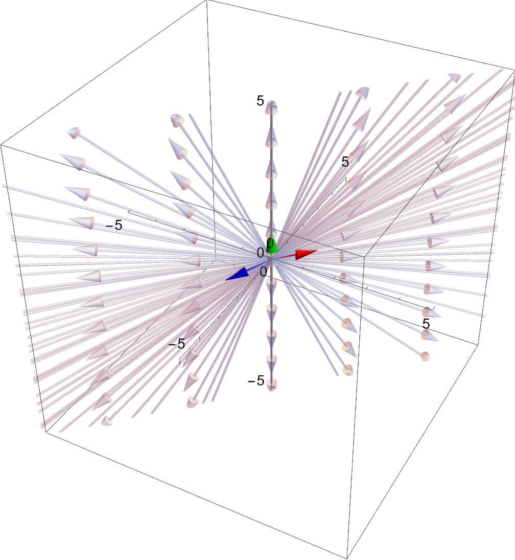
A span can also exist in 3 dimension. The following is the span of $\{\hat{\imath},\hat{\jmath},\hat{k}\}$


Linear dependence in three dimensions can result to spans that describe a **plane**:
$$
\{
\begin{bmatrix}
1\\1\\0
\end{bmatrix},
\begin{bmatrix}
0.5\\0.5\\0
\end{bmatrix},
\begin{bmatrix}
0\\0\\1
\end{bmatrix}
\}
$$


And spans that describe a **line**:
$$
\{
\begin{bmatrix}
1\\1\\0
\end{bmatrix},
\begin{bmatrix}
0.5\\0.5\\0
\end{bmatrix},
\begin{bmatrix}
-1\\-1\\0
\end{bmatrix}
\}
$$


### Linear Transformations and Matrix Multiplication

A **transformation** is basically a function that converts one vector to another vector. For example the transformation **$f$** can be defined as $f(\vec{x})=3\vec{x}$. Where a vector is just scaled to $3$. The domain of a transformation is usually, the span of $\{\hat{\imath},\hat{\jmath},\cdots\}$ or the entire $n$ dimensional vector space. You can think of a transformation visually as the **distortion** of the entire vector space. Applying a transformation to a vector is basically distorting the space the vector resides in.


Applied with a shear distortion


#### Liner Transformations

**Linear Transformations** are special transformations where the distortion of the vector space follows these rules:

1. The origin should not move
2. Parallel lines stay parallel
3. Straight lines stay straight

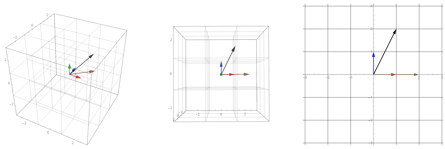
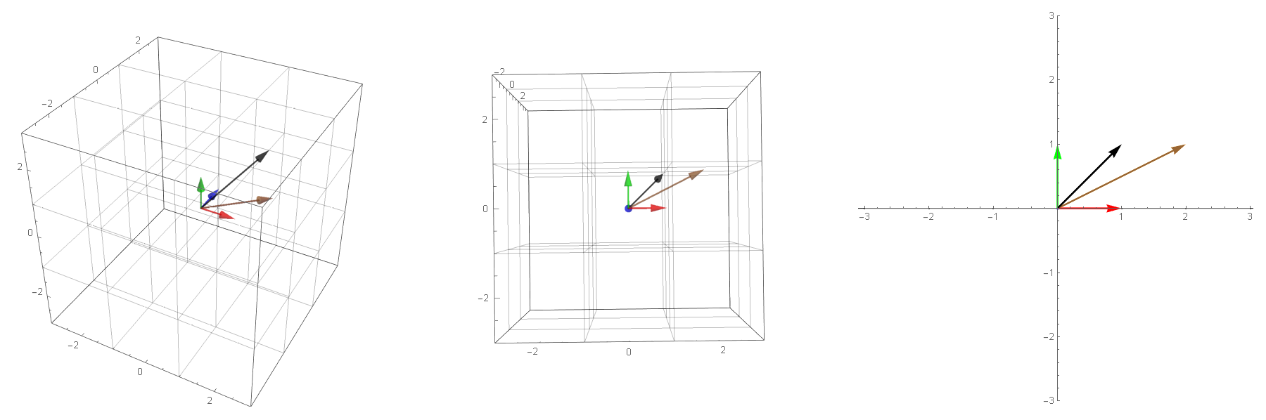
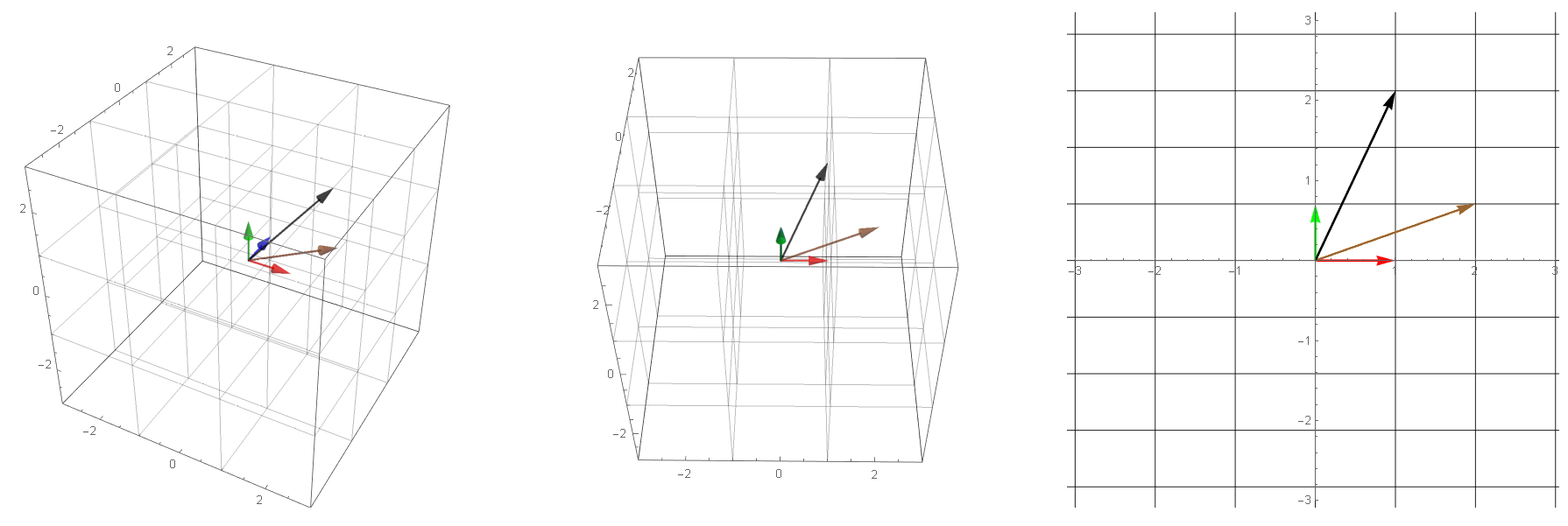
It turns out all transformations that satisfy the above rules can be perfectly described by watching how the **basis vectors** are transformed. For example the two plots below show a 90 degree rotation transformation.


- new $\hat{\imath}$ (red vector) :$\hat{\imath}'=\begin{bmatrix}0\\1\end{bmatrix}$

- new $\hat{\jmath}$ (blue vector): $\hat{\jmath}'=\begin{bmatrix}-1\\0\end{bmatrix}$

- Green vector: $1\begin{bmatrix}0\\1\end{bmatrix}+1\begin{bmatrix}-1\\0\end{bmatrix}=\begin{bmatrix}-1\\1\end{bmatrix}$

- Brown vector: $2\begin{bmatrix}0\\1\end{bmatrix}+1\begin{bmatrix}-1\\0\end{bmatrix}=\begin{bmatrix}-1\\2\end{bmatrix}$

- Yellow vector: $-2\begin{bmatrix}0\\1\end{bmatrix}+0.5\begin{bmatrix}-1\\0\end{bmatrix}=\begin{bmatrix}-0.5\\-2\end{bmatrix}$

- Black vector: $1\begin{bmatrix}0\\1\end{bmatrix}+-2\begin{bmatrix}-1\\0\end{bmatrix}=\begin{bmatrix}2\\1\end{bmatrix}$

All of the other vector values after the transformation is basically **scaled versions** of the new basis vectors in the same way that the pretransformed vector values are combinations of the original basis vectors. This means that any 2-dimensional linear transformation can be represented by 4 numbers, which we can write as a **matrix**, where each column corresponds to a basis vector. For this 90 degree rotation:

$$
T=\begin{bmatrix}
0&-1\\
1&0
\end{bmatrix}
$$

Any linear transformation is represented by the general matrix:

$$
T=\begin{bmatrix}
a&b\\
c&d
\end{bmatrix}
$$

#### Linear Transformation and Matrix Multiplication

Because of this, for any given transformation, we can easily find the output of the transformation for an arbitrary input vector using this formula:

$$
x\begin{bmatrix}
a\\
c
\end{bmatrix}+
y\begin{bmatrix}
b\\
d
\end{bmatrix}=
\begin{bmatrix}
ax+by\\
cx+dy
\end{bmatrix}
$$

Which is the exact result we get when we perform matrix multiplication:

$$
\begin{bmatrix}
a&b\\
c&d
\end{bmatrix}
\begin{bmatrix}
x\\
y
\end{bmatrix}=
\begin{bmatrix}
ax+by\\
cx +dy
\end{bmatrix}
$$

This ultimately means that all linear transformations can be defined as

$$
f(\vec{v})=T\vec{v}
$$

Other examples of linear transformations:

##### Horizontal Stretch

$$
T=\begin{bmatrix}
2&0\\
0&1
\end{bmatrix}
$$



##### Vertical Stretch

$$
T=\begin{bmatrix}
1&0\\
0&2
\end{bmatrix}
$$


##### Horizontal Shear

$$
T=\begin{bmatrix}
1&1\\
0&1
\end{bmatrix}
$$



##### Vertical Shear

$$
T=\begin{bmatrix}
1&0\\
1&1
\end{bmatrix}
$$



##### flip with respect to x-axis

$$
T=\begin{bmatrix}
1&0\\
0&-1
\end{bmatrix}
$$



#### Three Dimensional Transformations

Transformations also work similarly in 3 dimensions. The transformation below shows a shear on the yz direction.

$$
T=\begin{bmatrix}
1&1&1\\
0&1&0\\
0&0&1
\end{bmatrix}
$$


##### Composing transformations

You can combine transformations by performing transformations in a **sequence**. For example, you can **combine** a horizontal stretch with a vertical stretch which can be defined as a new transformation.


Since you are applying one transformation after the other, the overall transformation can be defined as a **composition** of the horizontal stretch transformation inside a vertical stretch transformation.

$$
\begin{aligned}
f(\vec{v})=\begin{bmatrix}
2&0\\0&1
\end{bmatrix}\vec{v}\\
g(\vec{v})=\begin{bmatrix}
1&0\\0&2
\end{bmatrix}\vec{v}\\
\\
g(f(\vec{v}))=\begin{bmatrix}
1&0\\0&2
\end{bmatrix}\Bigg(\begin{bmatrix}
2&0\\0&1
\end{bmatrix}\vec{v} \Bigg)
\end{aligned}
$$

The overall transformation can be achieved by applying horizontal stretch to $v$ first, then applying vertical stretch to the result of horizontal stretching.

Also if we record the final positions of the basis vectors after both stretchings, we can define a new matrix to represent the composition of both stretching.

$$
g(f(\vec{v}))=\begin{bmatrix}
1&0\\0&2
\end{bmatrix}\Bigg(\begin{bmatrix}
2&0\\0&1
\end{bmatrix}\vec{v} \Bigg)=
\begin{bmatrix}
2&0\\0&2
\end{bmatrix}\vec{v}
$$

What this actually shows is that matrix multiplication is associative since it turns out that:

$$
\begin{bmatrix}
1&0\\0&2
\end{bmatrix}\begin{bmatrix}
2&0\\0&1
\end{bmatrix}=\begin{bmatrix}
2&0\\0&2
\end{bmatrix}
$$

This means that any composition of transformations defined by matrices $T_1$ and $T_2$ can be summarized into the product $T_2T_1$.

$$
\begin{aligned}
f(\vec{v})&=T_1\vec{v}\\
g(\vec{v})&=T_2\vec{v}\\
g(f(\vec{v}))&=T_2T_1\vec{v}
\end{aligned}
$$

It is important to note, that although, matrix multiplication is associative, it is still not commutative. Which means the order of transformations matter. For example. A rotate and shear transformation will lead you to this transformation:


But a shear and rotate transformation will lead you this transformation:


##### Determinant

One of the important things you can study about a given linear transformation is how it generally **stretches** or **compresses** the space. For example, consider the linear transformation, horizontal stretching:

$$
T=\begin{bmatrix}
2&0\\
0&1
\end{bmatrix}
$$


Notice how the grid squares change in size and shape:


And for some arbitrary transformation:


The factor stretching/compression of the entire space that occurs during a transformation has a special name called the **determinant** of a transformation. The determinant is usually denoted as: $\det(T)$

The formula for the determinant of an arbitrary $2 \times 2$ transformation matrix $T$

$$
\begin{aligned}
T&=\begin{bmatrix}
a&b\\
c&d
\end{bmatrix}\\
\det\Bigg(\begin{bmatrix}
a&b\\
c&d
\end{bmatrix}\Bigg)&=ad-bc
\end{aligned}
$$

This formula can be derived by calculating the **area** of the resulting yellow parallelogram, which is the transformed version of the yellow square. This is because the area of the original grid is equal to 1.

The determinant of a 3 dimensional transformation is the factor of stretching/compression of the **volume** of the unit cube to the parallelepiped:



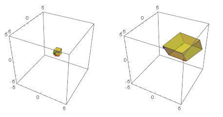
The factor of stretching/shrinking in any linear transformation.


The determinant of a 3x3 matrix can be calculated using Laplace expansion:

$$
\begin{aligned}
\det\Bigg(\begin{bmatrix}
a&b&c\\
d&e&f\\
g&h&i
\end{bmatrix}\Bigg)\\=a\det\Bigg(\begin{bmatrix}
e&f\\
h&i
\end{bmatrix}\Bigg)-
b\det\Bigg(\begin{bmatrix}
d&f\\
g&i
\end{bmatrix}\Bigg)+
c\det\Bigg(\begin{bmatrix}
d&e\\
g&h
\end{bmatrix}\Bigg)
\end{aligned}
$$

Consider the the following transformation:


This transformation has the corresponding matrix:

$$
\begin{bmatrix}
-1&2\\
1&1
\end{bmatrix}
$$

Which interestingly has the determinant

$$
\det\Bigg(\begin{bmatrix}
-1&2\\
1&1
\end{bmatrix}\Bigg)=-1(1)-2(1)=-3
$$

This means that the factor of stretching/compression for the transformation is **$-3$**. The **sign** of the determinant has meaning. If the determinant is negative it means that the space is **compressed beyond 0** to the point that the space is flipped.


Flipping space in the 3 dimensions means that the basis vectors cannot follow **right hand rule**.



##### Inverse Matrices

Consider the following system of linear equations:

$$
\begin{aligned}
2x+0y=4\\
0x+y=3
\end{aligned}
$$

This system of linear equation can be packaged into a single vector operation this way:

$$
\begin{bmatrix}
2&0\\
0&1
\end{bmatrix}
\begin{bmatrix}
x\\
y
\end{bmatrix}=
\begin{bmatrix}
4\\
3
\end{bmatrix}
$$

By writing a system of linear equation this way. You can think of the **coefficients** for $x$ and $y$ as the numbers that make up the **transformation matrix**, $T$. And you can think of the values on the right hand side of the equation as the result of the transformation matrix, $\vec{v}'$. This means that the solutions for the system of linear equations is the vector $\vec{v}$ which was the original value for $\vec{v}'$ before the transformation $T$.

$$
T\vec{v}=\vec{v}'
$$

To find the solutions of this system of linear equations, you need to look for the **original value** of $\vec{v}'$ **before** the transformation


To do this you need to make use of a special matrix related to the transformation matrix $T$, called the **inverse matrix**, $T^{-1}$. This matrix serves as the inverse of the transformation $T$ such that, **combining $T$ and $T^{-1}$** results to the original locations of the basis, or the identity matrix. Or:

$$
T^{-1}T=I
$$

For the example above the transformation is a horizontal stretch. By applying a horizontal shrink after a stretch, you get back to the original locations of the basis vectors:

$$
\begin{bmatrix}
0.5&0\\
0&1
\end{bmatrix}
\begin{bmatrix}
2&0\\
0&1
\end{bmatrix}=
\begin{bmatrix}
1&0\\
0&1
\end{bmatrix}
$$

This means that to solve the system of linear equations, you just need to apply the inverse transformation to $\vec{v}'$:

$$
\begin{aligned}
T^{-1}T\vec{v}=T^{-1}\vec{v}'\\
\vec{v}=T^{-1}\vec{v}'
\end{aligned}
$$

Using our example:

$$
\begin{bmatrix}
0.5&0\\
0&1
\end{bmatrix}
\begin{bmatrix}
4\\
3
\end{bmatrix}=
\begin{bmatrix}
x\\
y
\end{bmatrix}\\
\begin{bmatrix}
2\\
3
\end{bmatrix}=
\begin{bmatrix}
x\\
y
\end{bmatrix}
$$


###### Finding the inverse matrix

First you need to write your matrix augmented with identity matrix like this. As an example lets use a $3 \times 3$ matrix:

$$
\left[
\begin{array}{ccc|ccc}
3&0&2&1&0&0\\
1&-2&2&0&1&0\\
-1&3&2&0&0&1
\end{array}
\right]
$$

The goal here is to use some predefined rules to change your transformation matrix the identity matrix. Here are the rules:

1. You can change the values of a row by multiplying all of the numbers in the row by a constant
2. You can change rows by adding the elements of other rows to it.

First we need to focus on changing the values of the first column to make it follow the inverse matrix:

$$
\left[
\begin{array}{ccc|ccc}
(3)&0&2&1&0&0\\
1&-2&2&0&1&0\\
-1&3&2&0&0&1
\end{array}
\right]
$$

We can multiply the first row by $\frac{1}{3}$.

$$
\left[
\begin{array}{ccc|ccc}
1&0&\frac{2}{3}&\frac{1}{3}&0&0\\
1&-2&2&0&1&0\\
-1&3&2&0&0&1
\end{array}
\right]
\tag{$R_1\to \frac{1}{3}R_1$}
$$

To change the value of row 2, col 1 to 0, we need to multiply the $R_1$ by $-1$ and add it to $R_2$. We choose $R_1$ for this because we know that the value on row 1 col 1 is 1.

$$
\left[
\begin{array}{ccc|ccc}
1&0&\frac{2}{3}&\frac{1}{3}&0&0\\
0&-2&\frac{4}{3}&-\frac{1}{3}&1&0\\
-1&3&2&0&0&1
\end{array}
\right]
\tag{$R_2\to -R_1+R_2$}
$$

Next is to change $R_3$ by simply adding $R_1$ to it

$$
\left[
\begin{array}{ccc|ccc}
1&0&\frac{2}{3}&\frac{1}{3}&0&0\\
0&-2&\frac{4}{3}&-\frac{1}{3}&1&0\\
0&3&\frac{8}{3}&\frac{1}{3}&0&1
\end{array}
\right]
\tag{$R_3\to R_1+R_3$}
$$

We have completed the first column so we move to the second. Since row 1 col 2 is already 0, we move to row 2 col 2. And multiply $-\frac{1}{2}$ to the whole row to make it 1.

$$
\left[
\begin{array}{ccc|ccc}
1&0&\frac{2}{3}&\frac{1}{3}&0&0\\
0&1&-\frac{2}{3}&\frac{1}{6}&-\frac{1}{2}&0\\
0&3&\frac{8}{3}&\frac{1}{3}&0&1
\end{array}
\right]
\tag{$R_2\to -\frac{1}{2}R_2$}
$$

To finish this column we need to add the $-3R_2$ to the 3rd row to change the 3 to a zero. We choose the 2nd row because row 2 col 2 is now equal to 1.

$$
\left[
\begin{array}{ccc|ccc}
1&0&\frac{2}{3}&\frac{1}{3}&0&0\\
0&1&-\frac{2}{3}&\frac{1}{6}&-\frac{1}{2}&0\\
0&0&\frac{14}{3}&-\frac{1}{6}&\frac{3}{2}&1
\end{array}
\right]
\tag{$R_3\to -3R_2+R_3$}
$$

We now move on to the third column and change it to $\frac{14}{3}$ to 1. (You must always start by changing to 1 for each column so that changing to 0 is easier). We do this by multiplying it by $\frac{3}{14}$.

$$
\left[
\begin{array}{ccc|ccc}
1&0&\frac{2}{3}&\frac{1}{3}&0&0\\
0&1&-\frac{2}{3}&\frac{1}{6}&-\frac{1}{2}&0\\
0&0&1&-\frac{1}{28}&\frac{9}{28}&\frac{3}{14}
\end{array}
\right]
\tag{$R_3\to \frac{3}{14}R_3$}
$$

Next, we multiply $R_3$ by $-\frac{2}{3}$ and add it to $R_1$.

$$
\left[
\begin{array}{ccc|ccc}
1&0&0&\frac{5}{14}&-\frac{3}{14}&-\frac{1}{7}\\
0&1&-\frac{2}{3}&\frac{1}{6}&-\frac{1}{2}&0\\
0&0&1&-\frac{1}{28}&\frac{9}{28}&\frac{3}{14}
\end{array}
\right]
\tag{$R_1\to -\frac{2}{3}R_3+R_1$}
$$

Finally, we just need to multiply $R_3$ by $\frac{2}{3}$ and add it to $R_2$.

$$
\left[
\begin{array}{ccc|ccc}
1&0&0&\frac{5}{14}&-\frac{3}{14}&-\frac{1}{7}\\
0&1&0&\frac{1}{7}&-\frac{2}{7}&\frac{1}{7}\\
0&0&1&-\frac{1}{28}&\frac{9}{28}&\frac{3}{14}
\end{array}
\right]
\tag{$R_2\to \frac{2}{3}R_3+R_2$}
$$

The matrix on the right is the inverse of the original matrix

$$
\begin{bmatrix}
\frac{5}{14}&-\frac{3}{14}&-\frac{1}{7}\\
\frac{1}{7}&-\frac{2}{7}&\frac{1}{7}\\
-\frac{1}{28}&\frac{9}{28}&\frac{3}{14}
\end{bmatrix}
$$


###### Finding Inverses using the Cofactor Matrix

The inverse matrix can also be found using the cofactor matrix. To find the cofactor we use must first define the following matrix concepts:

###### Minors and Cofactors

The **minor** of some element $a_{ij}$ of a square matrix $A$, denoted by $M_{ij}$ is the determinant of the submatrix formed by deleting the $i$th row and $j$th column of $A$. Given a 3x3 matrix, we can find the three minors $M_{11}$, $M_{12}$, and $M_{13}$ as:
$$
\begin{aligned}
A &= \begin{bmatrix}
a&b&c\\
d&e&f\\
g&h&i
\end{bmatrix}\\
M_{11} &= \det(\begin{bmatrix}
e&f\\
h&i
\end{bmatrix})\\
M_{12} &= \det(\begin{bmatrix}
d&f\\
g&i
\end{bmatrix})\\
&\vdots\\
M_{33} &= \det(\begin{bmatrix}
a&b\\
d&e
\end{bmatrix})\\
\end{aligned}
$$

The **cofactor** of some element $a_{ij}$ of a square matrix $A$, denoted by $C_{ij}$ is calculated as:

$$
\begin{aligned}
C_{ij}=(-1)^{i+j}M_{ij}
\end{aligned}
$$

The **cofactor matrix** $C$ of some matrix $A$ is the matrix of $A$'s cofactors $C_{ij}$:

$$
\begin{aligned}
C = \begin{bmatrix}
C_{11}&C_{12}&C_{13}\\
C_{21}&C_{22}&C_{23}\\
C_{31}&C_{32}&C_{33}
\end{bmatrix}
\end{aligned}
$$

Using the cofactor matrix, we can calculate some the inverse $A^{-1}$ as:

$$
\begin{aligned}
A^{-1} = \frac{1}{\det(A)}C^{T}
\end{aligned}
$$

Using the previous example:

$$
\begin{aligned}
A &= \begin{bmatrix}
3&0&2\\
1&-2&2\\
-1&3&2
\end{bmatrix}\\
A^{-1} &=\frac{1}{\det(A)}C^T\\
\end{aligned}
$$

$$
\begin{aligned}
A^{-1} &=\frac{1}{\det(A)}C^T\\
A^{-1} &=\frac{1}{-28}\begin{bmatrix}
-10 & -4 & 1 \\
6 & 8 & -9 \\
4 & -4 & -6 \\
\end{bmatrix}^T\\
A^{-1} &= \begin{bmatrix}
\frac{5}{14} & -\frac{3}{14} & -\frac{1}{7} \\
\frac{1}{7} & -\frac{2}{7} & \frac{1}{7} \\
-\frac{1}{28} & \frac{9}{28} & \frac{3}{14} \\
\end{bmatrix}
\end{aligned}
$$

###### Singular Matrices

Most of the time solving systems of linear equations give you a single answer. But this is not always the case. There are three possibilities for this:

1. There is one solution
2. There are infinitely many solutions
3. There are no solutions

Possibilities 2 and 3 are special cases. These happen when the span of the transformed basis vectors (also called **column space**) has reduced dimension. For example, consider the following transformation matrix:

$$
T=\begin{bmatrix}
-1&2\\
0.5&-1
\end{bmatrix}
$$

If the transformed vector $\vec{v}'$ is not on the line described by the column space of $T$:

$$
\begin{aligned}
\begin{bmatrix}
-1&2\\
0.5&-1
\end{bmatrix}
\begin{bmatrix}
x\\
y
\end{bmatrix}=
\begin{bmatrix}
-1\\
3
\end{bmatrix}
\end{aligned}
$$


Then there are no solutions. On the other hand you may get lucky and the transformed vector $\vec{v}'$ may fall in the column space of $T$.

One way to check if a matrix is singular is by calculating the determinant. Since a singular transformation **collapses** the space from an $n$-dimensional span to $m$-dimensional span (where $m<n$), the space is shrunk to 0. Therefore, any singular matrix will have a **determinant of zero**. Using the previous example, we find that

$$
\begin{aligned}
\det\begin{bmatrix}
-1&2\\
0.5&-1
\end{bmatrix} = (-1)(-1)-(2)(0.5) = 0
\end{aligned}
$$



Then the system has infinitely many solutions. We call non-invertible matrices such as the aforementioned transformation above, **singular**.

#### Matrices in the Perspective of Linear Algebra

The main thesis of this series of lectures should not just be on the definitions of **matrices and their concepts**. The focus of this lecture is the essence of these concepts both **numerically** and **visually**. That's when we talk about matrix concepts, we always relate it linear transformations. It is not a coincidence that a matrix, an arbitrary collection of numbers arranged in a particular way, is related to linear transformations. In fact that is what a matrix is, a linear transformation.

Let's summarize what we know about vectors and matrices specifically in the perspective of linear transformations.

- A **vector** - an arbitrary member of some vector space, presented as an arrow from origin to a corresponding point in some $n$-dimensional space.
- An $n$-dimensional **square matrix** - defines some linear transformation, its values correspond to the new location of the basis vectors after the transformation.
- **matrix multiplication** - composition of linear transformations. The product summarizes the linear transformations into one.
- **determinant** - the factor of scaling of the vector space during a transformation
- **matrix inverse** - the functional inverse of a matrix, reverses the transformation

##### Non-square Matrices

Let's talk about a class of matrices we haven't talked about before, a **non-square matrix**:

$$
\begin{bmatrix}
2&2&-3 \\
-2& 1 & 0
\end{bmatrix}
$$

Matrices that look like this doesn't appear to fall into any of the linear algebra concepts we have discussed so far. But the closest related concept for these matrices are **linear transformations**. If these are indeed linear transformations, these matrices are meant to be **multiplied** to other vectors to apply some transformation.

$$
\begin{bmatrix}
2&2&-3 \\
-2& 1 & 0
\end{bmatrix}
\vec{v} = \vec{v}'
$$

Since this is a $2 \times 3$ matrix, you can only multiply these with vectors of size **$3 \times 1$**. But the interesting thing about this transformation is that it produces a vector of size **$2 \times 1$**.

$$
\begin{bmatrix}
2&2&-3 \\
-2& 1 & 0
\end{bmatrix}
\begin{bmatrix}
2\\
0\\
1
\end{bmatrix} = \begin{bmatrix}
1\\
-4
\end{bmatrix}
$$


From this we could gain an intuition about the special property of non-square matrices. It is also a linear transformation, but it is specifically a transformation that **changes** the number of dimensions of the vector space. There is some similarity between the transformation above and the transformation below:

$$
\begin{bmatrix}
2& 2& -3 \\
-2& 1& 0 \\
0& 0& 0&
\end{bmatrix}
\begin{bmatrix}
2\\
0\\
1
\end{bmatrix} = \begin{bmatrix}
1\\
-4 \\
0
\end{bmatrix}
$$


But the results of the transformation is actually different, the vector:

$$
\begin{bmatrix}
1\\
-4 \\
0
\end{bmatrix}
$$

is a three dimension vector, it just so happens that its $z$-axis component is zero. It still resides in the three dimensional vector space. On the other hand, the vector

$$
\begin{bmatrix}
1\\
-4
\end{bmatrix}
$$

Is a two dimensional vector which resides in the two dimensional vector space. They look the same but are not identical. Which means that:

$$
\begin{bmatrix}
1\\
-4 \\
0
\end{bmatrix} \neq \begin{bmatrix}
1\\
-4
\end{bmatrix}
$$

The transformation of any $n$-dimensional vector to less than $n$-dimensional space, is similar to producing the **projection** or shadow of the vector. Here are some interesting examples:

$$
T = \begin{bmatrix}
1&0&0 \\
0& 1 & 0
\end{bmatrix}
$$


$$
T = \begin{bmatrix}
1 & 0 & 0 \\
0 & 0 & 1
\end{bmatrix}
$$


$$
T = \begin{bmatrix}
1&0&0 \\
0& \frac{\sqrt{2}}{2} & \frac{\sqrt{2}}{2}
\end{bmatrix}
$$


You can also transform a **2-dimensional** vector into a **3-dimensional vector**, to do this you need a $3 \times 2$ transformation matrix.

$$
\begin{bmatrix}
3& 0\\
-1& -2\\
2& 1
\end{bmatrix}
\begin{bmatrix}
1\\
2
\end{bmatrix} = \begin{bmatrix}
3\\
-5\\
4
\end{bmatrix}
$$


As you can see above, even though the two dimensional vectors now reside in the three dimensional vector space, **the span that the basis vectors produce is still 2 dimensional**. This is because there is no way for the vectors to be transformed with **extra dimensionality**.

As a general rule, you can think of any $m \times n$ matrix as a transformation that transforms an **$n$-dimensional** vector into an **$m$-dimensional vector**.

#### Scalar products

The most well-known definition of a scalar product (also known as dot product) that you can find is the following:

> The scalar product of $\vec{a}$ and $\vec{b}$, denoted by $\vec{a} \cdot{} \vec{b}$ is the product of the magnitude of $\vec{a}$ and the magnitude of the projected version of $\vec{b}$ onto $\vec{a}$.

This is visually represented by the following dot products:
$$
\vec{b}\cdot{}\vec{g} = \vec{g}\cdot{}\vec{b}
$$


Which is calculated in the following manner:

$$
\begin{bmatrix}
a\\
b\\
\vdots\\
c
\end{bmatrix} \cdot
\begin{bmatrix}
x\\
y\\
\vdots\\
z
\end{bmatrix} = ax+by+\cdots+cz
$$

It is the measure of **similarity** between two vectors, For example, given three vectors,

$$
\vec{a}=\begin{bmatrix}
1\\
2\\
\end{bmatrix},
\vec{b}=\begin{bmatrix}
1\\
2.5\\
\end{bmatrix},
\vec{c}=\begin{bmatrix}
2\\
1\\
\end{bmatrix}
$$

Is $\vec{a}$ **more similar** to $\vec{b}$ or to $\vec{c}$?


$\vec{a}$ And $\vec{b}$ is more similar compared to $\vec{a}$ and $\vec{c}$:

$$
\begin{aligned}
\vec{a}\cdot{}\vec{b}=6\\
\vec{a}\cdot{}\vec{c}=4
\end{aligned}
$$

This means that two vectors perpendicular to each other will have a scalar product of **zero** and two vectors pointing in the opposite direction will have a **negative** scalar product:


These definitions are well and good, but unsatisfying for the thesis of this lecture. How does the scalar product relate to **linear transformations**?

We can construct a different definition for the scalar product, in the perspective linear transformation. And it turns out, a scalar product is merely a transformation of any vector to **one-dimensional space**:

The following dot product:

$$
\begin{bmatrix}
u_x\\
u_y\\
\end{bmatrix} \cdot{}
\begin{bmatrix}
a\\
b\\
\end{bmatrix} = u_xa+u_yb
$$

produces the same result as the following transformation:

$$
\begin{bmatrix}
u_x& u_y
\end{bmatrix}
\begin{bmatrix}
a\\
b\\
\end{bmatrix} = u_xa+u_yb
$$

This concept works for vectors of any number of dimensions. When looking at, the scalar product of two $n \times 1$ vectors, you can imagine that one vector is **reduced** into the **one dimensional vector space**. Which is similar to projecting it onto the line described by the other vector.

#### Eigenvectors and Eigenvalues

Consider the following transformation:

$$
\begin{bmatrix}
3& 1\\
0&2
\end{bmatrix}
$$



During the transformation most of the vectors change directions (i.e. the vector gets knocked from its span). Some special vectors however, just get scaled after the transformation. The vectors above colored green are just scaled versions of their input vector.

$$
\begin{aligned}
\begin{bmatrix}
3& 1\\
0&2
\end{bmatrix}
\begin{bmatrix}
-1\\
1
\end{bmatrix} &=
\begin{bmatrix}
-2\\
2
\end{bmatrix}=
2\begin{bmatrix}
-1\\
1
\end{bmatrix}\\ \begin{bmatrix}
3& 1\\
0&2
\end{bmatrix}
\begin{bmatrix}
1.5\\
0
\end{bmatrix} &=
\begin{bmatrix}
4.5\\
0
\end{bmatrix}=
3\begin{bmatrix}
1.5\\
0
\end{bmatrix}
\end{aligned}
$$

These special vectors are called **eigenvectors**. Each eigenvector is always accompanied by special scalar values called **eigenvalues**, which correspond to the factor of scaling for the transformation.

In fact **all** the vectors along the **span of the green vectors** are eigenvectors as well.




Based on how eigenvectors are defined, we can derive the process to find them. For any arbitrary transformation, eigenvectors are calculated by finding the vector solutions for the following inequality. Since eigenvectors are vectors that are **only** scaled as a result of the transformation, we can solve for $\vec{e}$ in the following equality. The scalar value **$\lambda$** refers to the unknown eigenvalue.

$$
T\vec{e}=\lambda\vec{e}
$$

Scalar times vector multiplication $\lambda \vec{e}$ can be written as a **linear transformation** instead. The effect of multiplying, $\lambda$ to $\vec{e}$, is exactly the same as **multiplying $\lambda I$ to $\vec{e}$**.

$$
\begin{bmatrix}
\lambda& 0& \cdots& 0\\
0& \lambda& \cdots& 0\\
\vdots& \vdots& \ddots& \vdots\\
0& 0& \cdots& \lambda
\end{bmatrix}
\vec{e}
$$

To solve for the unknowns, we can rewrite $T\vec{e}=\lambda\vec{e}$ into a s**olution from zero**:

$$
\begin{align*}
T\vec{e}&=\lambda I\vec{e}\\
T\vec{e}-\lambda I\vec{e}&=\vec{0}\\
(T-\lambda I)\vec{e}&=\vec{0}\\
\end{align*}
$$

If you recall, a non-zero vector can only be transformed to zero if and only if the whole vector space has been **squished to zero itself**. And this can only happen when the **determinant** of transformation is **zero**.

$$
\det(T-\lambda I)=\det(\begin{bmatrix}
t_{11}-\lambda& t_{12}& \cdots& t_{1n}\\
t_{21}& t_{22}-\lambda& \cdots& t_{2n}\\
\vdots& \vdots& \ddots& \vdots\\
t_{n1}& t_{n2}& \cdots& t_{nn}-\lambda
\end{bmatrix}) = 0
$$

This means that we can find the eigenvalues of any transformation by finding the **lambdas** that reduces the determinant to **$0$**. On a two dimensional vector, this is straightforward:

$$
\begin{aligned}
\det(\begin{bmatrix}
a-\lambda& b\\
c& d-\lambda
\end{bmatrix})=0\\
(a-\lambda)(d-\lambda)-bc=0
\end{aligned}
$$

Revealing the eigenvalues makes solving for the eigenvectors straightforward. Using the example above:

$$
\begin{aligned}
\det(\begin{bmatrix}
3-\lambda& 1\\
0& 2-\lambda
\end{bmatrix})&=0\\
(3-\lambda)(2-\lambda)-(1)(0)&=0\\
(3-\lambda)(2-\lambda)&=0\\
\\
\lambda &=2\\
\lambda &=3
\end{aligned}
$$

Since we know the eigenvalues, we can plug this back into the original equality, and solve the system of linear equations to find all the eigenvectors.

$$
\begin{aligned}
\begin{bmatrix}
3& 1\\
0&2
\end{bmatrix}
\vec{e} &=
2\vec{e}\\
\begin{bmatrix}
3& 1\\
0&2
\end{bmatrix}
\vec{e} &=
3\vec{e}
\end{aligned}
$$

$$
\begin{aligned}
\text{Eigenvectors for } &\lambda=2\\
3x +y &=2x\\
2y &= 2y\\
x+y&=0\\
x&=-y\\
&\begin{bmatrix}
u\\
-u
\end{bmatrix}
\end{aligned}
$$

$$
\begin{aligned}
\text{Eigenvectors for } &\lambda=3\\
3x+y &=3x\\
2y &= 3y\\
y&=0\\
&\begin{bmatrix}
v\\
0
\end{bmatrix}
\end{aligned}
$$

As you can see, the solutions for $\vec{e}$ is infinitely many, any vector of the form **$\begin{bmatrix}u\\-u\end{bmatrix}$** and any vector of the form **$\begin{bmatrix} v\\0\end{bmatrix}$** is an eigenvector.

#### Positive Definite Matrices and Positive Semidefinite Matrices

A symmetric matrix $A$ is said to be positive **semidefinite** if the scalar value $v^T A v$ is a positive number

#### Orthogonal Matrices

Square matrices where the corresponding basis vectors are exactly $90^{\circ}$ apart and their lengths are exactly 1 unit. Any orthogonal matrix $A$ satisfies the following condition:
$$
\begin{aligned}
A^{T} = A^{-1}
\end{aligned}
$$