---
date: 3 March 2020
category: CMSC57
description: If you happen to have zero background on what we are going to talk about in this series of topics, you might find it strange how a college course in computer science teaches you about counting.
---

# Counting and Discrete Probability

## Counting

If you happen to have zero background on what we are going to talk about in this series of topics, you might find it strange how a college course in computer science teaches you about counting. Although this lecture is indeed related to the concepts of cardinality, (how many things are there), we instead go deeper into slightly more complicated "*how many*" questions.

### Basic Rules of Counting

Counting **combinations** of related things become more interesting. Suppose you have a two **disjoint** sets of things called **$A$** and **$B$**, how do you count the number of **unique combinations** of the elements of **$A$** and **$B$**?

##### The Product Rule

Given a procedure with two tasks, if there are **$n_1$** ways to perform the first task and **$n_2$** ways to perform the second task, then there are **$n_1 n_2$** ways to perform the whole procedure.

For example, let **$A=\{a,b,c,d\}$**, **$B=\{x,y,z\}$**, if you list down **all** of the **possible combinations** this way:

| | **$a$** | **$b$** | **$c$** | **$d$** |
| :--: | :--: | :--: | :--: | :--: |
| **$x$** | **$ax$** | **$bx$** | **$cx$** | **$dx$** |
| **$y$** | **$ay$** | **$by$** | **$cy$** | **$dy$** |
| **$z$** | **$az$** | **$bz$** | **$cz$** | **$dz$** |

Since there are **$|A|=4$** columns and **$|B|=3$** rows, then there are **$(4)(3)$** unique combinations.

This can be generalized into **$|S_1|=n_1$** rows and **$|S_2|=n_2$** columns. Therefore the number of unique combinations are indeed **$n_1 n_2$**.

###### Examples

- How many unique plate number combinations can you produce out of the pattern: 3 letters and 3 numbers.
- How many unique 8-bit strings can be formed
- How many ways can you place 2 unique rings in your ten fingers?
- How many functions are there if the domain has **$u$** elements and the range has **$v$** elements?
- How many injective functions are there if the domain has **$u$** elements and the range has **$v$** elements?

As demonstrated in the first example, the product rule can be **extended**, to not just for two tasks. For a procedure composed of **$m$** tasks, **$T_1$**, **$T_2$**, **$T_3$**, ..., **$T_m$**, the number of ways to perform the whole procedure is **$n_1 n_2 n_3 \cdots n_m$**.

Supposing you have two disjoint sets again, **$A$** and **$B$**, how many things of either **$A$** or **$B$** are there?

##### Sum Rule

If a task can be done **either** in one of **$n_1$** ways or in **$n_2$** ways, (supposing each way is unique), there are **$n_1 + n_2$** ways to perform the specific task.

For example let let **$A=\{a,b,c,d\}$**, **$B=\{x,y,z\}$**, the cardinality of the **$|A \cup B|$** is simply **$|A| + |B| - |A \cap B|$**. Since **$A$** and **$B$** are assumed to be disjoint (because each way is supposed to be unique), then we simply add the cardinalities of the two sets **$A$** and **$B$**.

###### Examples

- If each character of a password can either be a letter, number, or an underscore. How many different ways can one character be.
- How many unique passwords of length 5 can you create?
- How many unique passwords of length 5-8 can you create?

> If we remove the assumption that the set of ways are disjoint, all we have to do is to subtract the cardinality of their intersection.

##### Subtraction Rule

If a task can be done either in one of **$n_1$** ways or in **$n_2$** ways and there are **$m$** ways common between two sets of ways, there are **$n_1 + n_2-m$** ways to perform the specific task.

- If **$H$** is the set of horror movies, **$T$** is the set of thriller movies and **$D$** is the set of drama movies. How many movies are either horror, thriller, or drama?

While there is product, sum and subtraction rule, there is also a division rule, This rule is used when some of the ways can be categorized as one.

##### Division Rule

If a task can be carried out **$n$** ways but there are exactly **$d$** identical ways for every unique way, there are **$\frac{n}{d}$** unique ways.

###### Example

- How many ways can you label four corners of a square with the labels, **$\{A,B,C,D\}$**? Assuming no labels can repeat and that rotating the labels along the corners does not create a unique labelling?

## Permutations and Combinations

Some of the examples that were described in the previous sections relate to a particular types of **counting problems**. Counting problems like two rings on ten fingers (where you can't put two rings on the same finger), the number of unique injections from some domain and range, 4-base pair sequences containing all 4 base pairs. These counting problems involve counting the number of **arrangements** and **combinations**. As it turns out problems like these have a lot of interesting aspects:

### Permutations

Permutation problems answer counting problems about unique arrangements. For example:

> How many ordered 3-tuples (where none of the elements repeat) can you describe from a set of 5 objects?

Since we are counting **tuples** (not subsets), the **order** of the elements matter (i.e. **$(a,b,c)\neq(b,a,c)$**.

We can answer this counting problem by dividing the it into three tasks, selecting which element resides in position 1 (5 ways, since there are 5 elements to choose from), selecting which element resides in position 2 (4 ways, since there are 4 elements to left), and selecting which element resides in position 3 (3 ways since there are 3 elements left). This gives the solution via product rule, **$5(4)(3)$**.

A **permutation** of a set of objects, is an ordered tuple (where each element is pairwise distinct) of the objects. An **$r$-permutation** on the other hand, is an ordered tuple (where each element is pairwise district) of any size **$r$** subset of the set.

For example given the set **$S=\{a,b,c,d\}$**, **$(a,b,c,d)$** and **$(a,c,b,d)$** are some permutations of **$S$**. The ordered tuple **$(a,c,d)$** is a 3-permutation of **$S$**, and **$(b,d)$** is a 2-permutation of **$S$**.

The number of **$r$**-permutations of any given set with **$n$** elements is denoted by **$P(n,r)$** or **$^nP_r$**. We can derive the general formula for **$P(n,r)$** using the product rule.

> If **$n$** is a positive integer and **$r$** is an integer where **$1\leq r\leq n$**.
> $$
> P(n,r)=n(n-1)(n-2)\cdots(n-r+1)
> $$

This multiplication can actually be neatly summarized using factorials, as shown below:

> $$
> \begin{aligned}
> P(n,r)&=\frac{n!}{(n-r)!}\\
> P(n,r)&=\frac{n(n-1)(n-2)\cdots(n-r+1)(n-r)(n-r-1)(n-r-2)\cdots(1)}{(n-r)(n-r-1)(n-r-2)\cdots(1)}
> \end{aligned}
> $$
>
> The product **$(n-r)(n-r-1)(n-r-2)\cdots(1)$** gets cancelled out leaving:
>
> $$
> P(n,r)=n(n-1)(n-2)\cdots(n-r+1)
> $$

Examples:

- How many ways can you award the first, second and third price in contest with 50 participants.
- How many different poker hands (5 cards) where the order matters are there in a deck of 52.

### Combinations

A combination is related to a permutation but with one major difference. While a permutation is associated to an ordered tuple, a combination is associated to a **subset**. It answers these types of questions:

> How many subsets of size 3 can you describe from a set of 5 objects?

Since we are now counting subsets we need to take note that **set equality** behaves differently. The order of the elements in a set doesn't matter (i.e. **$\{a,b,c\}=\{b,a,c\}$**).

To answer this counting problem, all we need to do is to apply the **division** rule after calculating the number of permutations:

> $$
> \begin{aligned}
> S&=\{a,b,c,d,e\}\\\\
> \{a,b,c\}&\to\Bigg\{
> \begin{matrix}
> (a,b,c)\\
> (b,c,a)\\
> \vdots\\
> (b,a,c)\\
> \end{matrix}\\
> \end{aligned}
> $$
>
> $$
> \begin{aligned}
> \{b,c,d\}&\to\Bigg\{
> \begin{matrix}
> (b,c,d)\\
> (c,d,b)\\
> \vdots\\
> (d,c,b)\\
> \end{matrix}\\
> \end{aligned}
> $$
>
> $$
> \begin{aligned}
> &\vdots\\
> \\
> \{c,d,e\}&\to\Bigg\{
> \begin{matrix}
> (c,d,e)\\
> (d,c,e)\\
> \vdots\\
> (e,c,d)\\
> \end{matrix}
> \end{aligned}
> $$

Since one combination is actually equivalent to **$P(3,3)$** permutations. We simply divide the total amount of 3-permutations by **$P(3,3)$**. Which is **$\frac{60}{6}=10$** combinations. This gives us the formula for **$r$-combinations** from a set of **$n$** elements:

> $$
> \begin{aligned}
> C(n,r)&=\frac{P(n,r)}{P(r,r)}\\
> C(n,r)&=\frac{\frac{n!}{(n-r)!}}{\frac{r!}{(r-r)!}}\\
> C(n,r)&=\frac{n!}{r!(n-r)!}
> \end{aligned}
> $$

The number of **$r$** combinations in a set of **$n$** elements has, is denoted as **$C(n,r)$**. It also usually denoted using **${n\choose r}$**

Examples:

- In a 6/42 lottery ticket, you select a set of **$6$** positive integers from a set of **$42$** positive integers. How many unique lottery tickets are there?
- Given a sorted list 6 unique numbers, how many sorted sublists are there
- How many bit strings of length 7 are there with exactly 3 zeroes?
- In the binomial expansion of **$(x+y)^3$**, what is the coefficient of **$x^2y$**.

### Binomial Theorem

Looking back at the previous example, we can see how we are able to use combinatorial truths to figure out the coefficient of a term in the expansion of the binomial **$(x+y)^3$**. As it turns out the same reasoning can be used for any binomial expansion **$(x+y)^n$**.

In the following binomial, the expansion is found by adding all possible combinations of **$x$**'s and **$y$**'s from all **$(x+y)$**.

$$
(x+y)^n=\underbrace{(x+y)(x+y)\cdots(x+y)}_n
$$

You can imagine one of the terms in the expansion to be of the form,

$$
cx^iy^{n-i}=cu_1u_2\cdots u_n
$$

where **$u_i$** is either **$x$** or **$y$** and the coefficient **$c$** is the number of times the exact combination of **$x$** and **$y$** is repeated. Therefore, to figure out the coefficient of some arbitrary term **$x^iy^{n-i}$** in the binomial expansion, you just have to answer the combinatorial question:

> how many **$u_1u_2\cdots u_n$** are there where there are exactly **$i$** **$x$**'s?

This asks the same question as the following combinatorial question in the context of bit strings:

> how many bit stings of length **$n$** are there with exactly **$i$** zeroes?

Which can be calculated using **$C(n,i)$**. Therefore, we can formulate the general form of any binomial expansion,

$$
\begin{aligned}
(x+y)^n&=\sum_{i=0}^{n}{{n \choose i}x^iy^{n-i}}\\
(x+y)^n&={n \choose 0}y^{n}+{n \choose 1}x^1y^{n-1}+\cdots+{n \choose n}x^n
\end{aligned}
$$

> For the first and the last element's **$x^0$** and **$y^0$** are ommited.

The binomial theorem can be used to algorithmically calculate the coefficients of an expansion with really large coefficients. For example the coefficient of the term **$x^{21} y^{13}$** of the binomial **$(x+y)^{34}$**:

$$
{34 \choose 21}x^{21}y^{13}=927983760x^{21}y^{13}
$$

The binomial theorem can answer interesting question about binomials an combinatoric forms,

> What is the sum of all coefficients in the expansion of a binomial on the **$n$th** degree?

This can be easily answered by calculating the following sum:

$$
\begin{aligned}
\sum_{i=0}^{n}{n \choose i}&=\sum_{i=0}^{n}{n \choose i}1^i 1^{n-i}\\
\sum_{i=0}^{n}{n \choose i}&=(1+1)^n\\
\sum_{i=0}^{n}{n \choose i}&=2^n
\end{aligned}
$$

Which actually make sense if you answer the question using the product rule since you there are 2 ways (selecting either **$x$** or **$y$**) in each of the **$n$** tasks in the whole procedure. This also makes sense on the context of bit strings since there are exactly **$2^n$** unique bit strings of length **$n$**.

The binomial theorem can lead us to more interesting corollaries related to combinatoric summations,

$$
\begin{aligned}
\sum_{i=0}^{n}{(-1)^i{n \choose i}}&=\sum_{i=0}^{n}{n \choose i}(-1)^i 1^{n-i}\\
\sum_{i=0}^{n}{(-1)^i{n \choose i}}&=(-1+1)^n\\
\sum_{i=0}^{n}{(-1)^i {n \choose i}}&=0^n=0
\end{aligned}
$$

### Pascals Identity and Triangle

One more important principle related to binomial coefficients is **Pascal's triangle**. You may have encountered this principle in during high school algebra but this time we are approaching it in the context of combinatorics.

One of the most important combinatoric identities is known as **Pascal's Identity**:

$$
{n+1 \choose r}={n \choose r-1}+{n \choose r}
$$

The identity can be proven algebraically in the following way:

$$
\begin{aligned}
{n \choose r-1}+{n \choose r}&=\frac{n!}{(r-1)!(n-(r-1))!}+\frac{n!}{r!(n-r)!}\\
&=\frac{n!}{(r-1)!(n-r+1)!}+\frac{n!}{r!(n-r)!}\\
&=\frac{n!r}{r!(n-r+1)!}+\frac{n!(n-r+1)}{r!(n-r+1)!}\\
&=\frac{n!r+n!(n-r+1)}{r!(n-r+1)!}\\
&=\frac{n!(n+1)}{r!(n+1-r)!}\\
&=\frac{(n+1)!}{r!(n+1-r)!}\\
{n \choose r-1}+{n \choose r}&={n+1 \choose r}
\end{aligned}
$$

This identity actually proves the mechanism behind Pascal's triangle

$$
\begin{matrix}
&&&&&&&1&&&&&&\\
&&&&&&1&&1&&&&&\\
&&&&&1&&2&&1&&&&\\
&&&&1&&3&&3&&1&&&\\
&&&1&&4&&6&&4&&1&&\\
&&1&&5&&10&&10&&5&&1&\\
&1&&6&&15&&20&&15&&6&&1
\end{matrix}
$$

$$
\begin{matrix}
&&&&&&&{0 \choose 0}&&&&&&\\
&&&&&&{0 \choose 0}&&{0 \choose 0}&&&&&\\
&&&&&{2 \choose 0}&&{2 \choose 1}&&{2 \choose 2}&&&&\\
&&&&{3 \choose 0}&&{3 \choose 1}&&{3 \choose 2}&&{3 \choose 3}&&&\\
&&&{4 \choose 0}&&{4 \choose 1}&&{4 \choose 2}&&{4 \choose 3}&&{4 \choose 4}&&\\
&&{5 \choose 0}&&{5 \choose 1}&&{5 \choose 2}&&{5 \choose 3}&&{5 \choose 4}&&{5 \choose 5}&\\
&{6 \choose 0}&&{6 \choose 1}&&{6 \choose 2}&&{6 \choose 3}&&{6 \choose 4}&&{6 \choose 5}&&{6 \choose 6}
\end{matrix}
$$

## Finite Probability Space

One of the first mathematicians to explore the concept of probability was the French mathematician Pierre-Simon Laplace. He studied the concept under the context of gambling. He defined the probability of an event as the number of outcomes leading to that event, divided by the number of possible outcomes.

Let's start this topic by discussing some key terminologies:

- **experiment** - in the context of probability an experiment is a procedure that results to exactly one outcome out of a set of possible outcomes.
- **sample space** - we call the set of possible outcomes of a particular experiment its corresponding sample space
- **event** - an event is a subset of the sample space

Using laplace's definition:

> if **$S$** is a **finite** nonempty sample space of equally likely outcomes, and **$E$** is an event, given that **$E \subset S$**, The probability of event **$E$**, (denoted by **$p(E)$**):
>
> $$
> p(E)=\frac{|E|}{|S|}
> $$

The probability of an event can only be between **$0$** to **$1$**. That is because the **$E$** is a subset of **$S$**. Therefore, we can conclude that its cardinality is greater than or equal to **$0$** and less than or equal to **$|S|$** ($0 \leq |E| \leq |S|$).

For example, given a box that contains 3 oranges, 6 apples, and 2 bananas, what is the probability that a fruit chosen at random from the box is an **orange**?

To answer this question, we first identify what is the sample space and what is the event. The sample space in this experiment is the set of eleven fruits, 3 of them are oranges and 6 of them are apples, and two of them are bananas. The event that we are concerned with is the event that chooses an orange. Since there are 3 oranges, the probability for choosing an orange can be calculated as: **$\frac{3}{11}$**.

###### Examples

- Given the same scenario above, what is the probability that two fruits selected at random are both bananas?

- What is the probability that a ticket wins the 6/49​ lottery? Selecting a combination of 6 numbers from 1 to 49.
- After uniformly shuffling the list **$[3,2,1,1,4,5]$**, what is the probability that the shuffling produces a sorted list?

#### Probabilities of unions of events

If your looking for the probability that either one of two events **$E$** or **$F$** occurs (where both **$E$** and **$F$** are subsets of **$S$**), you can simply combine the two events into one event which corresponds to their union. Since this union is still the subset of the sample space **$S$**, you can use Laplace's definition to find the probability:

$$
\begin{aligned}
p(E \cup F) &= \frac{|E|+|F|-|E \cap F|}{|S|}\\
&= \frac{|E|}{|S|}+\frac{|F|}{|S|}-\frac{|E \cap F|}{|S|}\\\\
p(E \cup F) &= p(E) + p(F) + p(E \cap F)
\end{aligned}
$$

#### Probabilities of complements

If the probability of an event is known, finding the probability that said event doesn't occur is very easy. We can leverage the fact that since event **$E$** is a subset of **$S$**, then the set difference **$S-E$** (which is also a subset of **$S$**), corresponds to all events where **$E$** is not the outcome. That is because **$S-E$** is literally the set of all outcomes that are not **$E$**. This leads us to the formula for the probability of the **complement** of an event, (denoted by **$p(\overline{E})$**):

$$
\begin{aligned}
p(\overline{E}) &= p(S-E)\\
&=\frac{|S-E|}{|S|}\\
&=\frac{|S|-|E|}{|S|}\\
&=1-\frac{|E|}{|S|}\\\\
p(\overline{E})&=1-p(E)
\end{aligned}
$$

This principle is very useful since there are times where the **complement** of an event is much **easier** to identify than the event itself. For example, solving for the probability of a random 8-bit string having at least one zero directly is tedious since you have to add the probabilities for the events where the string has one zero, two zeroes, three zeroes, and etc. If you instead identify the complement, which is the probability that a random 8-bit string has 8 ones, (zero zeroes, or the probability not of having at least one zero):

(Given **$E$** as the event where the random bit string has at least one zero)

$$
\begin{aligned}
p(E)&=1-P(\overline{E})\\
&=1-\frac{|\overline{E}|}{|S|}\\
&=1-\frac{1}{2^8}\\
&=1-\frac{1}{256}\\\\
p(E)&=\frac{255}{256}
\end{aligned}
$$

### Probability theory

Laplace's definition for the probability of an event in a finite sample space assumes that all possible outcomes have **equal** likelihood to occur. This cannot be assumed for all experiments in the **real world** since some outcomes are actually more likely than the others. A coin may be **biased** in such a way that outcome of flipping to one specific side is more likely, than the other side.

The definition for probability can be generalized for finite probability space experiments that **don't** have equally likely outcomes. This is done by assigning a specific probability **$p(s)$** for each outcome **$s \in S$**. The assignment of specific probabilities can only be valid if **$0 \leq p(s) \leq 1$** for each outcome **$s$**, and that **$\sum_{s \in S}{p(s)}=1$** (each probability is within the range **$[0,1]$**, and the sum of all probabilities is exactly **$1$**). By satisfying both conditions, an experiment is guaranteed to have exactly one outcome among the sample space.

This definition of probability describes the function, **$p:S\to [0,1]$**, known as the **probability distribution** for the particular experiment. The correct assignment of each probability **$p(S)$** should satisfy the limit:

$$
\lim_{n\to \infty}{\frac{u}{n}}=p(s)
$$

Given that after performing the experiment **$n$** times, the outcome **$s$** occurred **$u$** times. For example, as you increase the number of times you flip an unbiased coin, the ratio of flipping heads divided by the number of flips should approach **$\frac{1}{2}$**.

An example of proper assignments of probabilities look something like this:

> Given the sample space for flipping a coin, **$S=\{H,T\}$**:
>
> - **$p(H)=\frac{1}{2}$**
> - **$p(T)=\frac{1}{2}$**

A probability distribution such as the above which follows Laplace's assumption of having equally likely outcomes, is called a **uniform distribution**. This implies that a uniformly distributed experiment will have a probability assignment **$p(s)=\frac{1}{n}$** where **$s \in S$** and **$|S|=n$**.

This then gives us a more general definition for the probability of an event **$E$** as the sum of all the probabilities of the outcomes related to event **$E$**.

$$
p(E)=\sum_{s \in E}{p(s)}
$$

The formula for compound probabilities remain to be true in the general definition of probability:

- **$p(E_1 \cup E_2)=p(E_1)+p(E_2)-p(E_1 \cap E_2)$**
- **$p(\overline{E})=1-p(E)$**

#### Conditional Probability

Given a six-sided die, what is the probability that the sum of two rolls is **divisible by three**?

To answer this, all we need to do is to figure out the event that described above. Supposing the ordered pair **$(u,v)$** corresponds to the outcome rolling **$u$** and then rolling **$v$**, the event described above corresponds to the following set: **$\{(1,2),(2,1),(1,5),(5,1),(2,4),(4,2),(3,3)\}$**. Since each of the outcomes in this event have the probability **$\frac{1}{36}$**, the probability that the sum of two rolls is divisible by three is **$\frac{7}{36}$**.

How would the probability change, if we change the scenario, such that the first die roll is **$2$**?

A modified scenario like this asks for:

"the **conditional probability** of two rolls being divisible by three given that the first roll is 2"

A conditional probability is often denoted by **$p(E|F)$** where **$E$** is the desired event and **$F$** is the assumed event.

We can answer these probability questions by imagining a sample space where all first dice rolls are **$2$**, **$F=\{(2,1),(2,2),(2,3),(2,4),(2,5),(2,6)\}$**. We then look at the set of outcomes where both **$E$** and **$F$** is satisfied (the first roll is 2 and the sum of both rolls is divisible by three) or the set **$E \cap F=\{(2,1),(2,4)\}$**. This means that the **$E|F$** occurs 2 out of 6 times, giving us the conditional probability **$p(E|F)=\frac{1}{3}$**.

In general the formula for a conditional probability of $E$ given $F$ is:

$$
p(E|F)=\frac{p(E \cap F)}{p(F)}
$$

Let's look at another example, what is the probability that the second flip of a fair coin is heads given that the first flip is tails?

Given **$H$** as the event that the second flip is heads, and **$T$** as the event that the first flip is tails, we solve for **$p(H|T)$**:

$$
\begin{aligned}
p(H|T)&=\frac{p(H \cap T)}{p(T)}=\frac{\frac{1}{4}}{\frac{1}{2}}\\\\
p(H|T)&=\frac{1}{2}
\end{aligned}
$$

##### Independence

When considering conditional probabilities, the concept of probabilistic independence often comes up. When you think about it, the outcome of the first coin flip **does not actually affect** the outcome of the second coin flip. Knowing the outcome of the first coin flip will not give us any information about the outcome of the second coin flip. In fact you can remove the first roll out of the picture and restate the question as the following: **"*what is the probability of flipping a heads*"**. The probability of this event is exactly the same as the probability of **$p(H|T)$**. Whenever **$p(H|T)=p(H)$**, we can conclude that the events **$H$** and **$T$** are **independent**. This gives us the mathematical definition for independent events:

> **$E$** and **$F$** are independent if and only if **$p(E \cap F)=p(E)p(F)$
>
> **$p(E \cap F)=p(E)p(F)$** is just algebraic manipulation of **$p(E|F)=p(E)$**.

#### Bernoulli Trials and Binomial Distributions

Performing an experiment that can only have two outcomes (such as flipping a coin) has a special name, it is called a **Bernoulli trial**. Since the trial can only have two outcomes (generally called successes and failures), we can infer that the probability of successes, **$p$** and the probability of failures, **$q$** will sum up to 1, ($p+q=1$).

Bernoulli trials are special since there are a lot of problems that can be solved by determining the number of successes in a given amount of mutually independent trials.

Given **$p$** as the probability of success and **$q$** as the probability of failure in a trial, we can solve for the probability of having **$k$** successes in **$n$** mutually independent trials:

> When **$n$** trials is performed, there are a total of **$2^n$** possible outcomes. The number of ways exactly **$k$** successes appear in **$n$** trials is exactly **$C(n,k)$**. Since each of these ways have the probability **$p^k q^{n-k}$** (because each trial is mutually exclusive we can just multiply all probabilities). Therefore, the probability of having exactly **$k$** successes is:
>
> $$
> b(k;n,p)=C(n,k)p^k q^{n-k}
> $$
>
> The probability of a observing **$k$** successes in **$n$** mutually exclusive Bernoulli trials with probability success **$p$** is denoted by **$b(k;n,p)$**.

The probability **$b(k;n,p)$** as a function of **$k$** is called a **binomial distribution**.

Example:

What is the probability that a randomly generated 6-bit string has exactly 4 zeroes? (Assuming each digit is generated independently and the outcomes 1 and 0 have the same likelihood)

> Since the value of each digit in a 6-bit string is a independent from the other digits, and a digit can only be either a 0 (success) and a 1 (failure), we can restate this as the following probability: **$b(4,6,0.5)$**. Therefore, this probability is:
>
> $$
> b(4,6,0.5)=C(6,4)0.5^40.5^2=0.2345375
> $$

#### Bayes' Theorem

One of the most powerful theorems related to probability is the Bayes' theorem. Named after mathematician Thomas Bayes, this theorem comes up in inferential statistics, risk analysis, machine learning, natural language processing and many more. Bayes theorem assesses the probability that a particular event occurs based on some evidence.

Consider the following scenario:


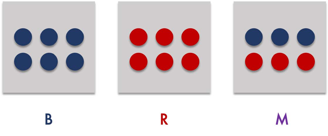
Consider three opaque boxes, lets call them B, R, and M. Box B has 6 blue balls, box R has 6 red balls and box and box M has 3 blue balls and 3 red balls. Suppose you select a box randomly:


What is the probability that the selected box is box B (lets call this **$p(B)$)? The answer is very straightforward, since box B is one event out of 3 possible outcomes in the sample space, the probability is **$\frac{1}{3}$**. In fact the selected box is equally likely to be box R or box M.

Suppose you pick a random ball in the selected box without looking inside and it turned out to be a blue ball. Lets call picking a blue ball **$b$**.


How does event **$b$** affect the probability that this box is box B? Does this increase or decrease the probability that this is box B?

This is guaranteed to not be box R since box R only has red balls. Only half of box M's contents are blue balls while all of box B's contents are blue balls. Because of that you can conclude the following:

$$
0=p(R|b)<p(M|b)<p(B|b)
$$

This is an example of the application of Bayesian reasoning. At the start of the scenario, we are able to calculate that the probability of the selected box being box B, is **$p(B)=\frac{1}{3}$**. We call this probability the **prior** probability (since the probability is before any evidence is gathered). After gathering some **evidence** by randomly picking a ball inside the selected box (event **$b$) we update our intuition about the probability of the selected box being B. We know denote this probability as **$p(B|b)$**. Which is the probability that the selected box is blue given that one of the balls inside is blue.

What exactly is **$p(B|b)$**? Before we answer that, let us derive Bayes' theorem by looking at a general scenario:

Given some event **$Q$**, and some evidence **$R$**, what is the probability of **$Q$** occurring after observing the evidence **$R$** (i.e. **$p(Q|R)$**), if evidence **$R$** occurs in **$Q$** with the probability **$p(R|Q)$**?

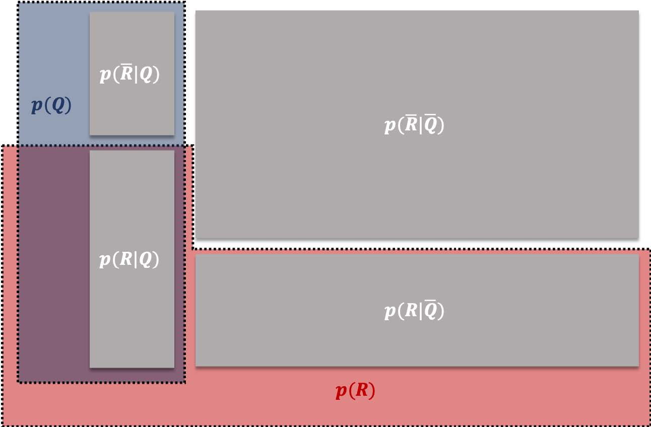
We can represent this general scenario using the following diagram:


$$
\begin{aligned}
P(Q) &= P(R|Q) + P(\overline{R}|Q)\\
\end{aligned}
$$

This diagram represents the probabilities of all possible events in the sample space. The sample space can be divided into two outcomes **$Q$** and **$\overline{Q}$** (either **$Q$** occurs or **$Q$** doesn't occur),


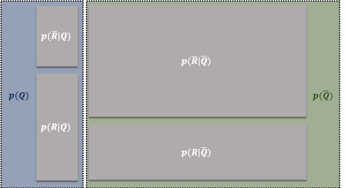
Within the outcome **$p(Q)$**, the evidence **$R$** has the probability of being observed as **$p(R|Q)$**. Therefore to figure out **$p(Q|R)$**, we just need to look at the proportion of the occurrences of **$R|Q$**, among all occurrences of **$Q$** in the sample space,


Suppose the size of the sample space is **$|S|$**, we can represent the total number of **$|Q|$** occurences as **$p(Q)|S|$**. That's because **$p(Q)$** is basically the ratio of **$|Q|$** occurences divided by all possible outcomes:

$$
\begin{aligned}
p(Q)&=\frac{|Q|}{|S|}\\
p(Q)|S|&=\frac{|Q|}{|S|}|S|\\\\
p(Q)|S|&=|Q|
\end{aligned}
$$

> You can think of **$|S|$** as the total area of the overall rectangle and **$p(Q)|S|$** as the total area of the two rectangles in the left side.

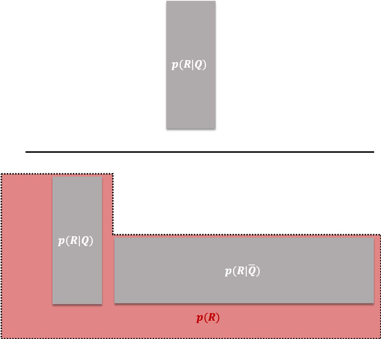
Using the same reasoning we can figure out the number of occurrences corresponding the event **$R|Q$**. Since there are **$p(Q)|S|$** occurrences where **$Q$** is the outcome, **$p(R|Q)p(Q)|S|$** is the number of occurrences corresponding the event **$R|Q$**. Also, with the same reasoning **$p(R|\overline{Q})p(\overline{Q})|S|$** is the number of occurrences corresponding the event **$R|\overline{Q}$**.

Therefore, the probability **$p(Q|R)$** can be calculated as:

$$
\begin{aligned}
p(Q|R)=\frac{p(R|Q)p(Q)|S|}{p(R|Q)p(Q)|S|+p(R|\overline{Q})p(\overline{Q})|S|}
\end{aligned}
$$

cancelling out **$|S|$** on the numerator and denominator gives us the definition of Bayes' theorem:

$$
\begin{aligned}
p(Q|R)=\frac{p(R|Q)p(Q)}{p(R|Q)p(Q)+p(R|\overline{Q})p(\overline{Q})}
\end{aligned}
$$

- **$p(Q|R)$** - the **posterior** probability, or the probability that Q occurs after observing evidence **$R$** occurred
- **$p(Q)$** - the **prior** probability, or the probability of **$Q$** before observing the evidence
- **$p(R|Q)$** - the **likelihood of the R given Q** or the probability of **$R$** occurring specifically on **$Q$** outcomes

> If the general probability of the evidence **$p(R)$** is known, the theorem can be written like the following:
>
> $$
> \begin{aligned}
> p(Q|R)=\frac{p(R|Q)p(Q)}{p(R)}
> \end{aligned}
> $$

To answer the question earlier, what exactly is the probability of the selected box being the box B, given that one of the balls is blue, or the posterior, **$p(B|b)$**?

- The prior probability **$p(B)=\frac{1}{3}$**.

- The likelihood of picking blue balls in box B is **$p(b|B)=1$**.

- The likelihood of picking blue balls in boxes that are not B (either R or M) can be calculated as, **$p(b|\overline{B})=p(b|R \cup M) = \frac{p(b \cap (R \cup M))}{p(R \cup M)} = \frac{1}{4}$**.

> **$\frac{1}{4}$** is calculated using the following lemma**: **$p(b \cap (R \cup M))= p(b|R)p(R)+p(b|M)p(M)$
>
> The proof of this lemma, (recall conditional probability)
>
> $$
> \begin{aligned}
> p(b|R)p(R)+p(b|M)p(M)&=\frac{p(b \cap R)}{p(R)}p(R)+\frac{p(b \cap M)}{p(M)}p(M)\\
> &=p(b \cap R)+p(b \cap M) - 0\\
> &=p(b \cap R)+p(b \cap M) - p((b \cap R) \cap (b \cap M))*\\
> &=p((b \cap R) \cup p(b \cap M))\\
> &=p(b \cap (R \cup M))
> \end{aligned}
> $$
> *$p((b \cap R) \cap (b \cap M))=0$** because a box cannot be both R and M at the same time, therefore there is zero probability that this intersection of events happens. I added this so that the use of union of events theorem is clearer.
>
> Therefore we get **$\frac{1}{4}$** like this:
> $$
> \begin{aligned}
> p(b|\overline{B})&=p(b|R \cup M)\\&=\frac{p(b \cap (R \cup M))}{p(R \cup M)}\\&=\frac{p(b|R)p(R)+p(b|M)p(M)}{p(R \cup M)}\\
> &=\frac{0(\frac{1}{3})+\frac{1}{2}(\frac{1}{3})}{\frac{2}{3}}\\
> p(b|\overline{B})&=\frac{3}{12}=\frac{1}{4}
> \end{aligned}
> $$
>

Therefore the posterior probability **$p(B|b)$**:

$$
\begin{aligned}
p(B|b)&=\frac{p(b|B)p(B)}{p(b|B)p(B)+p(b|\overline{B})p(\overline{B})}\\
p(B|b)&=\frac{1(\frac{1}{3})}{1(\frac{1}{3})+(\frac{1}{4})(\frac{2}{3})}\\\\
p(B|b)&=\frac{2}{3}
\end{aligned}
$$

Calculating the probabilites for other boxes supports our intuition earlier,

$$
\begin{aligned}
p(M|b)&=\frac{p(b|M)p(M)}{p(b|M)p(M)+p(b|\overline{M})p(\overline{M})}\\
p(M|b)&=\frac{(\frac{1}{2})(\frac{1}{3})}{(\frac{1}{2})(\frac{1}{3})+(\frac{1}{2})(\frac{2}{3})}\\\\
p(M|b)&=\frac{1}{3}\\\\
p(R|b)&=\frac{p(b|R)p(R)}{p(b|R)p(R)+p(b|\overline{R})p(\overline{R})}\\
p(R|b)&=\frac{(0)(\frac{1}{3})}{(0)(\frac{1}{3})+(\frac{3}{4})(\frac{2}{3})}\\\\
p(R|b)&=0
\end{aligned}
$$

##### Bayesian spam filters

On of the known applications of bayesian theorems is through probabilistic classification algorithms. The **naive bayes algorithm** uses the bayesian theorem to classify the classification of something based on its characteristics. This algorithm has been used in **bayesian spam** filters where an email can be classified as spam or not spam. Spam emails usually contain characteristic spam key words. The presence of these spam key words on an email provide evidence for the naive bayes algorithm that increases the likelihood for that email to be spam. These keywords are words that are learned by the algorithm by observing their occurences on known spam emails.

#### Random variable and expected value

The **expected value** of some random variable (some variable that represents the outcome of an experiment) represents the most likely value based on the probability distributions of all the possible outcomes. Identifying the expected value answers interesting questions about how the outcome of repeated experiments.

For example you might be interested in knowing the expected number of heads after flipping a coin 100 times. This can be identified by calculating the sum of all products of each outcome in the sample space times the probability of said outcome.

Assuming the coin is fair, one coin flip has two outcomes, heads or tails, so one coin flip can have either zero or one heads. If we imagine a random variable **$X$** that represents the number of heads in a coin flip, we know that this random variable **$X$** have two possible values, **$X=1$** or **$X=0$**. Therefore the expected value of canX be calculated as the following:

$$
\begin{aligned}
E(X)&=\sum_{s\in\{1,0\}}{p(s)s}\\
E(X)&=\frac{1}{2}(1)+\frac{1}{2}(0)\\\\
E(X)&=0.5
\end{aligned}
$$

> Where **$E(X)$** is the expected value of **$X$**

Meaning we expect that there are 0.5 heads in one coin flip which means there are 0.5(100) or 50 heads in 100 coin flips.

The expected value of a random variable can be thought of as the weighted mean value of a random variable where the weights are the probabilities assigned to each possible value.

Expected values are very useful in more interesting experiments such as the following example,

*What is the expected value of the sum of numbers that appears in a pair of dice?*

Since the outcome of each die is independent from the other, you can imagine this as two repetitions of on die roll. So the expected value is simply the expected value if one dice roll times 2:

$$
\begin{aligned}
E(X)&=\frac{1}{6}(1)+\frac{1}{6}(2)+\frac{1}{6}(3)+\frac{1}{6}(4)+\frac{1}{6}(5)+\frac{1}{6}(6)\\
E(X)&=\frac{1}{6}(21)\\
E(X)&=\frac{7}{2}\\\\
2(E(X))&=7
\end{aligned}
$$

> where **$X$** is the random variable that represents the outcome of a die roll.

##### Variance

Variance measures how spread out are the possible values of a random variable. This can be easily calculated as the the square of the expected difference between the mean and the random variable values:

$$
\text{Var}(X)=E((X-E(X))^2)
$$

This seems like a strange formula but if you imagine the squared difference **$(X-E(X))^2$** as a random variable, then you can calculate its expected value as the weighted average of squared deviations from the mean:

$$
\text{Var}(X)=\sum_{s \in S}p(s)(s-E(X))^2
$$