# Asymptotic Analysis
The way we're going to approach this topic is by getting directly into the definitions and mechanics.
You might not be able to immediately appreciate the reason why we are discussing these mathematical constructs.
They seem very unusual and appear to have nothing to do with computer science.
But rest assured that at the end of this topic I will be discussing the application of these particular constructs in computer science.
In fact, the reason why I decided to put this topic right at the start of the semester is because this topic is up there with the most important things you need to master as computer scientists.
As you mature as computer scientists you'll be able to apply these mathematical constructs from automatically, as if it's muscle memory.
You are going to spend a couple of weeks to master these concepts.
We're doing this so that you'll start your growth as computer scientists with strong mathematical and theoretical foundations.
## Formal Definitions
We'll jump right in with the formal definition of the constructs known as Big-O (Big-O), Big-$\Omega$ (Big-Omega), and Big-$\Theta$ (Big-Theta).
### Big-O
$$
\begin{aligned}
&O(g(n))=\{f(n)| \exists c>0,n_0>0\\
&(\forall n>n_0 (0 \leq f(n) \leq cg(n))) \}
\end{aligned}
$$
Now this definition looks very complicated indeed, but if you are unable to recall how mathematical expressions of sets and quantifications are interpreted, don't worry here's how you read this definition:
> _"**Big -Oh**"_ of some function $g(n)$ is the set of all functions $f(n)$, where there exists a positive constant $c$ such that $0 \leq f(n) \leq cg(n)$ for sufficiently large values of $n$ (for values of $n$ above some positive value $n_0$ ($n \geq n_0 \geq 0$)).
This definition, although now closer to English, is still quite a mouthful.
Let's dissect the meaning of this definition:
First the most important part of this definition is the inequality inside the set roster member notation:
$$
0 \leq f(n) \leq cg(n)
$$
According to the definition, any function of $n$, $f(n)$ is a member of the set known as $O(g(n))$ if it satisfies this inequality for all sufficiently large values of $n$ (or for all values of $n$ that are large enough).
The extra condition: "for all sufficiently large values of $n$" is manifested in the universal quantification $\forall n\geq n_0$.
What this means is that, **this inequality must hold true for all values $n$ that reach a threshold $n_0$**.
It doesn't matter which exact value $n_0$ is, all we know is that it is positive and it must exists ($\exists n_0 \geq 0$) for $f(n)$ to be a member.
Therefore, for a function of $n$ to be member of the set $O(g(n))$, **all images $f(n)$ must be not be greater than the corresponding image $g(n)$ times $c$**.
The constant $c$ is another positive number that must exist for this inequality.
_This whole definition will make much more sense with a visual example like the one below.
The function $13n + 2$ can be shown to be a member of the set $O(2n^2 + n)$_
$$
13n + 2 \in O(2n^2+n)
$$
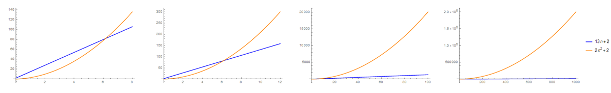
As shown in the plot, even though the function $13n+2$ starts bigger than $2n^2+n$, after some point, $2n^2+n$ **overtakes** the function $13n+2$ and leaves it behind so much that $13n+2$ is only barely visible on the last plot.
This shows that **there exists an $n_0$, a threshold for $n$, where, we are sure that for any $n$ greater than $n_0$, the inequality $13n+2 \leq 2n^2+n$ is always true**
In this example, the function $2n^2+n$ starts to overtake between $n=6$ and $n=7$.
We don't even have to know the exact value of this turning point point, we can just show that $n_0$ exists and it's value is $n_0=7$ (you can also not be conservative and use a bigger number like $n_0=100$ or $n_0=10000$).
After this point, we see that there will never be a value of $n$ greater than $n_0$ where $13n+2$ is greater than $2n^2+n$.
Also, it looks like we have not explicitly picked a value for $c$ in this example because the value is already true for $c=1$.
As long as we are able to show that this inequality will hold for at least one pair of positive values, $n_0$ and $c$ (in this case we picked $n_0=7$ and $c=1$), we are sure that $13n + 2$ is indeed a member of $O(2n^2+n)$.
_Let's hammer it home with another example.
One which forces us to explicitly choose a value for $c$_
$$
11n+1 \in O(2n+4)
$$
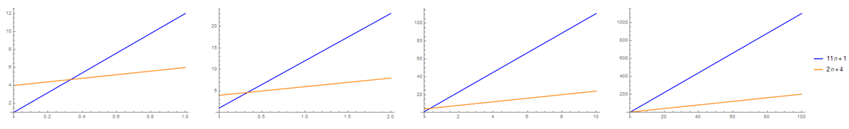
From the plots above you can see that **$2n+4$, starts bigger, but then $11n+1$ overtakes it around $n=0.4$**.
And beyond this point, $11n+1$ stays above $2n+4$, and based on the definition of Big-O this is evidence that $2n+4\in O(11n+1)$ (and this assertion is indeed true).
This evidence does not show us that $11n+1 \in O(2n+4)$.
But, if we choose a value for $c$, for example, $c = 10$, we get the following plot:
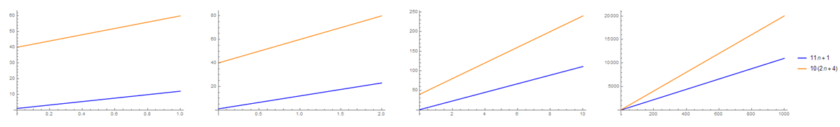
This shows that f**or $c=10$, the function $10(2n+4)$, starts as bigger than $2n+4$ and is always bigger than $2n+4$** (you can check that this is true if you notice that the difference between their values only gets bigger as $n$ increases).
Remember that if we just find at least one pair of positive numbers $n_0$ and $c$ (in this case $n_0=0, c=10$) that satisfy the inequality, we are able to conclude that $11n+1 \in O(2n+4)$.
It might seem strange that both $11n+1 \in O(2n+4)$ (where $n_0=0,c=10$) and $2n+4\in O(11n+1)$ is true (where $n_0=0.4,c=1$) but this is a legitimate possibility.
In fact two way relationships like this have a certain implication that will be discussed later.
_The relationship $13n + 2 \in O(2n^2+n)$ are usually read as the following phrases that you will repeatedly hear as computer scientists:_
- **$13n + 2$ is upper bounded by $O(2n^2+n)$** - it's called an upper bound because as $n$ increases to large values, $13n+2$ can never be greater than $2n^2 + n$.
There is a boundary above $13n+2$ and that boundary is $2n^2 + n$.
- **$13n + 2$ cannot be more complex than $2n^2 + n$** - the term complexity is often used when contextualized with programming.
When dealing with programming resources such as time, memory, and etc, CS often abstracts these resources as complexities (i.e.
time complexity, space complexity).
This will be discussed in detail later.
> _When we say $f(n)$ cannot be more complex than $g(n)$, it means that it is still possible that $f(n)$ is equally as complex as $g(n)$,_
### Big-$\Omega$
You can think of Big-$\Omega$ as the opposite of Big-O.
Here's the definition:
$$
\begin{aligned}
&\Omega(g(n))=\{f(n)| \exists c>0,n_0>0\\
&(\forall n>n_0 (0 \leq cg(n) \leq f(n))) \}
\end{aligned}
$$
Here's how this definition is interpreted:
> _"**Big -Omega**"_ of some function $g(n)$ is the set of all functions $f(n)$, where there exists a positive constant $c$ such that $0 \leq cg(n) \leq f(n)$ for sufficiently large values of $n$ (for values of $n$ above some positive value $n_0$ ($n \geq n_0 \geq 0$)).
You'll notice that the difference between this definition and the Big-O definition can be found on the inequality inside the set:
$$
0 \leq cg(n) \leq f(n)
$$
Here, **$cg(n)$ is now less than or equal to $f(n)$**.
The principles behind the definition of Big-O are the same principles that we use for the definition of Big-$\Omega$.
Instead of $f(n)$ getting upper bounded by $g(n)$, a Big-$\Omega$ relationship asserts that $f(n)$ is now lower bounded by $g(n)$.
This relationship looks more apparent with the following example:
$$
2n^3+10 \in \Omega(4n^2+30)
$$
The plot below demonstrates this assertion:
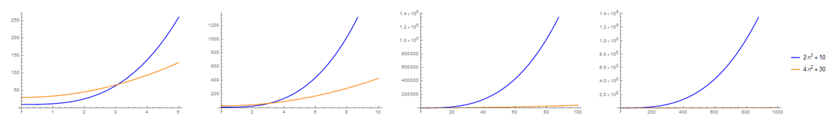
Here using $c=1$ we see that around $n=3.4$ the $2n^3 + 10$ starts to become bigger than $4n^2 + 30$.
After this point we are certain that $2n^3 + 10$ will never become smaller than $4n^2 + 30$, thus showing that $c$ and $n_0$ indeed exists in the form of $c=1,n_0=3.4$.
Showing that the relationship, $2n^3+10 \in \Omega(4n^2+30)$ is true.
Therefore we can say the following about the relationship between the functions $2n^3 + 10$ and $2n^3 + 10$:
- **$2n^3 + 10$ is lower bounded by $4n^2 + 30$.**
- **$2n^3 + 10$ cannot be less complex than $4n^2+30$.**
> _When we say $f(n)$ cannot be less complex than $g(n)$, it means that it is still possible that $f(n)$ is equally as complex as $g(n)$,_
### Big-$\theta$
The definition of Big-$\Theta$ is a like a combination of the definitions of Big-O and Big-$\Omega$
$$
\begin{aligned}
&\Theta(g(n))=\{f(n)| \exists c_1>0,c_2>0,n_0>0\\
&(\forall n>n_0 (0 \leq c_1g(n) \leq f(n) \leq c_2g(n))) \}
\end{aligned}
$$
This is how it's interpreted:
> _"**Big -Theta**"_ of some function $g(n)$ is the set of all functions $f(n)$, where there exists a positive constant $c_1$ and $c_2$ such that $0 \leq c_1g(n) \leq f(n) \leq c_2g(n)$ for sufficiently large values of $n$ (for values of $n$ above some positive value $n_0$ ($n \geq n_0 \geq 0$)).
In this definition, **the inequality conditions for Big-O and Big-$\Omega$ are combined into one**.
The value for $f(n)$ is between $c_1g(n)$ and $c_2g(n)$.
For a function to be shown as a member of $\Theta(g(n))$, we must demonstrate the existence of three positive numbers, $c_1$, $c_2$, and $n_0$.
When we establish that a function $f(n)=\Theta(g(n))$, we mean that $f(n)$ is tightly bound by $g(n)$ (we say this because it is both upper bounded and lower bounded, by $g(n)$).
Here's an example of this in action:
$$
4n^2+30 \in \Theta(2n^2 + n)
$$
_To demonstrate that this is indeed true, we just need to satisfy the inequality:_
$$
c_1(2n^2 + n) \leq 4n^2 + 30 \leq c_2(2n^2 + n)
$$
Basically, we need to show that $2n^2 + n$ can be upper bound and lower bound $4n^2 + 30$.
To do this we just need to select some appropriate coefficients, $c_1$ and $c_2$.
For this example we have found that to be $c_1=1$ and $c_2=3$.
This can be shown on the plot below:
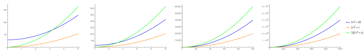
After some threshold $n_0$ notice how the $4n^2 + 30$ stays in between $2n^2+n$.
This is what it means for a function to be tightly bound to another.
The value of $2n^2 + n$ can be either greater or lesser than $4n^2 + 30$, it depends on the coefficients.
We can say the following about the relationship between $4n^2 + 30$ and $2n^2+n$:
- $4n^2 + 30$ is tightly bounded by $2n^2 + n$.
- $4n^2 + 30$ is as complex as $2n^2 + n$.
> Before we move on the next section, here are some questions to ponder upon: (don't worry, these questions will be answered and proven in the next sections)
>
> - **Is it true that $f(n) \in O(g(n)) \cup \Omega(g(n))$ for any pair of functions $f(n)$ and $g(n)$?** (_I.e.
> Is $f(n)$ guaranteed to be a member of either $O(g(n))$ or $\Omega(g(n))$?)_
> - **Is it true that if $f(n) \in O(g(n))$, then $g(n)\in \Omega(f(n))$?**
> - **What is $O(g(n)) \cap \Omega(g(n))$?** (_What is the intersection of $O(g(n))$ and $\Omega(g(n))$?_)
### Proving Asymptotic Relationships using the Formal Definition
Let's look at proving asymptotic relationships between two functions.
One of the things a computer scientist repeatedly does, is to establish the asymptotic relationship between two functions.
Questions such as: "**is $n^2 + 5 \in O(n^2)$?** ".
This task is done so ubiquitously and automatically that the techniques you'll end up using become so easy.
For now, we'll discuss the most basic technique of answering these questions.
For this part we'll use the definition of O, $\Omega$, and $\Theta$ to answer these questions.
_For example, let's prove that the relationship demonstrated visually in the previous sections, is indeed true:_
$$
2n^3+10 \in \Omega(4n^2+30)
$$
_Recall that the definition for a $\Omega$ relationship is the following:_
$$
\begin{aligned}
&\Omega(g(n))=\{f(n)| \exists c>0,n_0>0\\
&(\forall n>n_0 (0 \leq cg(n) \leq f(n))) \}
\end{aligned}
$$
We will use this definition to prove that the assertion above is true.
To do this, we just need to formally show what we demonstrated in the previous section.
That, $2n^3 + 10$ qualifies as a legitimate member of the set $\Omega(4n^2+30)$.
Therefore, we just need to show that the following is true:
$$
\begin{aligned}
&\exists c>0,n_0>0\\
&(\forall n>n_0 (0 \leq c(4n^2 + 30) \leq 2n^3 + 10)
\end{aligned}
$$
_We can satisfy the existential quantification above using proof by example with the following values:_
$$
\text{let } c = 1, n_0 = 3.4
$$
_and a little bit of inequality algebra:_
$$
\begin{aligned}
4n^2 + 30 &\leq 2n^3 + 10\\
4n^2 + 20 &\leq 2n^3\\
2 + \frac{10}{n^2} &\leq n\\
\end{aligned}
$$
Since we selected $n_0 = 3.4$.
The universal quantification is limited to n > 3.4.
This means that the value for $\frac{10}{n^2}$ cannot be greater than $\frac{10}{3.4^2}$ or approximately $0.865.$ This is because as $n$ increases, the fraction $\frac{10}{n^2}$ decreases.
Therefore, the left hand side of the inequality is the most competitive when $n=3.4$.
Any number greater than that will just decrease the left hand side, $2 + \frac{10}{n^2}$ (when $n$ becomes so large the lhs value approaches the value 2[^1]) while increasing the right hand side, $n$,
[^1]: In fact this is connected to how limit definitions work (which will be discussed in the next section) and why this whole concept is called **asymptotic** analysis.
#### Proving non-membership
**What if we needed to prove that a function is not a member of O, $\Omega$, or $\Theta$**? For example, how do we prove the following?
$$
2n^3+10 \notin O(4n^2+30)
$$
It's not as simple as using proof by example to demonstrate the existence of $c$ and $n_0$ that does not satisfy the inequality.
To begin this proof we first negate the quantification in the set definition of Big-O.
We just need to apply DeMorgan's law to it:
$$
\begin{aligned}
\neg &(\exists c>0,n_0>0\\
&(\forall n>n_0 (0 \leq (2n^3+10) \leq c(4n^2+30))))\\\\
&(\forall c>0,n_0>0\\
&(\exists n>n_0 (0 > (2n^3+10) \lor (2n^3+10) > c(4n^2+30)))
\end{aligned}
$$
> note: we do not actually care for cases where $n<0$ or $f(n)<0$ or in fact anything that is less than $0$.
> In the context that we are using this in computer science, values are cannot be negative.
With this negation we end up with a universal quantification that shows that **it is not enough to find a few values for $c$ and $n_0$**.
We should **prove that for all possible combinations of $c$ and $n_0$, sometimes there is a value for $n$ that is greater than $n_0$, that satisfies $(2n^3+10) > c(4n^2+30)$.**
The process to demonstrate this is similar to the process demonstrated above.
Starting with some inequality algebra:
$$
\begin{aligned}
2n^3+10 &> c(4n^2+30)\\
2n^3+10 &> 4n^2c+30c\\
n+\frac{10}{2n^2} &> 2c+\frac{30c}{2n^2}\\
n &> 2c+\frac{30c}{2n^2}-\frac{10}{2n^2}\\
\end{aligned}
$$
It looks like we ended up with a very strange inequality, but this is all we need.
The right hand side value, $2c+\frac{30c}{2n^2}-\frac{10}{2n^2}$, decreases as $n$ increases.
Again, this is because of the $n^2$ in the denominators of the fraction.
Now, **no matter what combination of $c$ and $n_0$, you choose, there will always be a value of $n$ that satisfies this because the left hand side (which is also $n$) increases as $n$ increases.** On the other hand, **the right hand side decreases as $n$ increases**.
This will always be satisfied no matter what humongous combination of $n_0$ and $c$ you choose because there will always be a value of $n$ that will surpass that.
## Limit Definitions
Now that we've been properly acquainted with the formal set definitions of O, $\Omega$ and $\Theta$.
Let's look at arguably more intuitive definitions, the limit definitions.
You'll need a little background in calculus to grasp the essence of this definition.
You don't really need to be an expert, you just need a little background on how limits and infinities work.
If you are keen you'll notice that this definition is not entirely brand new.
We've been informally introduced with this definition when we explored proving them membership and non-memberships of functions into certain O, $\Omega$, and $\Theta$, sets.
Written formally the limit definitions of asymptotic notation are the following:
$$
\begin{aligned}
\lim_{n \to \infty} \frac{f(n)}{g(n)} &<\infty \to f(n) \in O(g(n))\\
\lim_{n \to \infty} \frac{f(n)}{g(n)} &> 0 \to f(n) \in \Omega(g(n))\\
0<\lim_{n \to \infty} \frac{f(n)}{g(n)} &< \infty \to g(n) \in \Theta(f(n))\\
\end{aligned}
$$
These definitions sound complicated, but if we try to translate these into English, you'll realize that it actually does make sense.
The left hand sides (the limit) are read like the following
> if the limit of the ratio $\frac{f(n)}{g(n)}$ as $n$ approaches infinity...
We're looking at the ratio of the two functions $f(n)$ and $g(n)$ and **we're trying to see what happens to the value of that ratio as $n$ becomes very very large (as $n$ approaches infinity).**
### Approaching Infinity
Lets look at this with an example.
We'll use these functions:
$$
\begin{aligned}
f(n)&=2n^3+10 \\
g(n)&=4n^2+30
\end{aligned}
$$
If we use small numbers to substitute to $n$, the value of the ratio $\frac{2n^3+10}{4n^2+30}$ will not really help tell us about the relationship between $f(n)$ and $g(n)$:
$$
\begin{aligned}
&\text{Let }n=5\\
\\
&\frac{2(5)^3 + 10}{4(5)^2 + 30} = 5
\end{aligned}
$$
But as we **increase** the value of $n$, we'll notice that the **value of the ratio becomes bigger and bigger**:
$$
\begin{aligned}
&\text{Let }n=100\\
\\
&\frac{2(100)^3 + 10}{4(100)^2 + 30} \approx 50\\
\\\\
&\text{Let }n=1000\\
\\
&\frac{2(1000)^3 + 10}{4(1000)^2 + 30} \approx 500\\
\\\\
&\text{Let }n=100000\\
\\
&\frac{2(100000)^3 + 10}{4(100000)^2 + 30} \approx 50000\\
\end{aligned}
$$
We can expect this number to **increase** as we increase the value of $n$.
When we reach really big values of $n$, (around infinity), we can expect that that number will be **really** big as well.
And of course this behavior should happen.
That's because we are looking at the ratio between two values, positively dependent $n$.
It just so happens that the numerator of this fraction is of polynomial degree 3 while the denominator is of polynomial degree 2.
What this means is that the numerator of the ratio will increase much faster than the denominator.
When the value $n$ becomes really big, **the value of the numerator will become extremely big compared to the denominator**.
And what do we get when we divide a very big number by a relatively small number? A very big number.
Let's look at another pair of functions as an example:
$$
\begin{aligned}
f(n)&=13n + 2 \\
g(n)&=2n^2+n
\end{aligned}
$$
Using the same principle as above, we examine the effect of increasing the value of $n$ to the value of the ratio $\frac{13n+2}{2n^2+n}$:
$$
\begin{aligned}
&\text{Let }n=100\\
\\
&\frac{13(100) + 2}{2(100)^2 + 100} \approx 0.0647\\
\\\\
&\text{Let }n=10000\\
\\
&\frac{13(10000) + 2}{2(10000)^2 + 10000} \approx 0.000649\\
\\\\
&\text{Let }n=10000000\\
\\
&\frac{13(10000000) + 2}{2(10000000)^2 + 10000000} \approx 6.5 \times 10^{-7}\\
\end{aligned}
$$
As you observe here, as the value of $n$ increases, **the value of the ratio, becomes closer and closer to 0**.
We can expect that when we reach really big values, **the value of the ratio will be very close to zero**.
We expect this because the numerator is of degree 1 while the denominator is of degree 2.
As the value of $n$ increases, both the numerator increases but the denominator increases faster.
Therefore, when reaching very big values, we end up dividing a number over a relatively big number.
The result of this division is a value close to 0.
Now, instead of going through the trouble of testing for bigger and bigger numbers we can immediately figure out which one of the numerator or denominator is the relatively larger value.
This is where the limit towards infinity comes to play.
We directly look at the value of the ratio when the value of $n$ approaches to **infinity** (a very big value).
Using the same examples above:
$$
\lim_{n \to \infty} \frac{2n^3+10}{4n^2+30}
$$
If we directly substitute[^2] infinities to $n$ directly:
$$
\begin{aligned}
=&\frac{2(\infty) ^3+10}{4(\infty)^2+30}\\
=&\frac{\infty}{\infty}
\end{aligned}
$$
[^2]: Just to clarify: we are not actually substituting the value here, we are solving the limit, and to do that we conceptually substitute infinity to the variable $n$.
The fraction infinity over infinity is an undefined value, so instead of automatically substituting infinity to $n$, we'll need to apply **L'Hopital's rule** first:
$$
\begin{aligned}
\lim_{n \to \infty} \frac{2n^3+10}{4n^2+30} &= \lim_{n \to \infty} \frac{\frac{d}{dx}(2n^3+10)}{\frac{d}{dx}(4n^2+30)}\\
&= \lim_{n \to \infty} \frac{6n^2}{8n}\\
&= \lim_{n \to \infty} \frac{3n}{4}\\
\end{aligned}
$$
By applying L'Hopital's rule, we can now freely _substitute_, infinity to $n$, giving us:
$$
\lim_{n \to \infty} \frac{2n^3+10}{4n^2+30} = \lim_{n \to \infty} \frac{3n}{4} = \infty
$$
Therefore, based on the limit definitions, we can conclude that $2n^3+10 \in \Omega(4n^2+30)$.
If you don't know what L'Hopital's rule is, its basically a technique for solving otherwise undefined/indeterminate limit ratio values.
The exact usage of L'Hopital's rule is as follows:
$$
\lim_{n\to c}\frac{f(n)}{g(n)} = \lim_{n\to c}\frac{\frac{d}{dx}f(n)}{\frac{d}{dx}g(n)}
$$
Basically, if you are unable to solve limits (because you end up with undefined/indeterminate values like $\frac{0}{0}$, $\frac{\infty}{\infty}$), you derive both the denominator and numerator separately.
If after applying L'Hopital's rule, you still end up with undefined/indeterminate values, you can apply it again, until you get an answer that is either 0, some positive constant, or infinity.
Let's look at two more examples of this:
$$
\begin{aligned}
\lim_{n \to \infty} \frac{13n+2}{2n^2+n} &= \lim_{n \to \infty} \frac{\frac{d}{dx}(13n+2)}{\frac{d}{dx}(2n^2+n)}\\
&= \lim_{n \to \infty} \frac{13}{4n+1}\\
&=0
\\\\
\therefore 13n+2 &\in O(2n^2 +n)
\end{aligned}
$$
$$
\begin{aligned}
\lim_{n \to \infty} \frac{4n^3+3n^2}{6n^3+1} &= \lim_{n \to \infty} \frac{\frac{d}{dx}(4n^3+3n^2)}{\frac{d}{dx}(6n^3+1)}\\
&= \lim_{n \to \infty} \frac{12n^2+6n}{18n^2}\\
&= \lim_{n \to \infty} \frac{\frac{d}{dx}(12n^2+6n)}{\frac{d}{dx}(18n^2)}\\
&= \lim_{n \to \infty} \frac{24n+6}{36n}\\
&= \lim_{n \to \infty} \frac{\frac{d}{dx}(24n+6)}{\frac{d}{dx}(36n)}\\
&= \lim_{n \to \infty} \frac{24}{36}\\
\lim_{n \to \infty} \frac{4n^3+3n^2}{6n^3+1} &= 46\\
\\\\
\therefore 4n^3+3n^2 &\in \Theta(6n^3+1)
\end{aligned}
$$
Note how L'Hopital's rule had to be applied thrice to solve this.
Also, if we end up with a limit value between 0 and infinity (meaning any positive constant), This means that neither the numerator or denominator is relatively bigger than the other.
In cases like these, the numerator is a member of big theta of the denominator.
$$
\begin{aligned}
\lim_{n \to \infty} \frac{n \log_5 n +3n}{5n^2+4n+2} &= \lim_{n \to \infty} \frac{\frac{d}{dx}(n \log_5 n +3n)}{\frac{d}{dx}(5n^2+4n+2)}\\
&= \lim_{n \to \infty} \frac{n\frac{1}{n\ln 5} + \log_5 n + 3}{10n + 4}\\
&= \lim_{n \to \infty} \frac{\frac{d}{dx}(\frac{1}{\ln 5} + \log_5 n + 3)}{\frac{d}{dx}(10n + 4)}\\
&= \lim_{n \to \infty} \frac{\frac{1}{n\ln 5}}{10}\\
&= \lim_{n \to \infty} \frac{1}{10n(\ln5)}\\
\lim_{n \to \infty} \frac{n \log_5 n +3n}{5n^2+4n+2} &= 0
\\\\
\therefore n \log_5 n +3n &\in O(5n^2+4n+2)
\end{aligned}
$$
## Asymptotically Loose Relationships
You might be wondering why, we read asymptotic notation with the qualifier "Big", why do we have to specify **Big**-O, or **Big**-Omega? Well, you might have guessed it, its because there are "little" versions of O, and $\Omega$.
Both little-o and little-$\omega$ are what we call asymptotically loose relationships.
### Little-o
Starting with the set definition of little-o, it is defined as:
$$
o(g(n)) = \{f(n)|\forall c>0(\exists n_0>0(\forall n>n_0(0 \leq f(n) \leq cg(n))))\}
$$
> For all positive constants $c$, there exists a positive constant $n_0$, such that $0 \leq f(n) \leq cg(n)$ for all $n>n_0$, (for sufficiently large values of $n$)
This definition is sort of a stricter version of Big-O, where instead of just proving the existence of $c$ that will make the inequality true, we have to prove that the inequality is true for all possible values of $c$.
Here's the limit definition of little-o:
$$
\lim_{n \to \infty} \frac{f(n)}{g(n)} = 0 \to f(n) \in o(g(n))
$$
Compared to Big-O, where the value of the limit must jut be anything less than infinity, for a little-o relationship to be true, the value of the limit must be exactly zero.
An example of this relationship is:
$$
5n^2 + 3n \in o(2n^3)
$$
### Little-$\omega$
The definition of little-$\omega$ is as follows:
$$
\omega(g(n)) = \{f(n)|\forall c>0(\exists n_0>0(\forall n>n_0(0 \leq cg(n) \leq f(n))))\}
$$
> For all positive constants $c$, there exists a positive constant $n_0$, such that $0 \leq cg(n) \leq f(n)$ for all $n>n_0$, (for sufficiently large values of $n$)
This is similarly a strict version of Big-$\Omega$, where we also need to prove that the inequality is true for all possible positive constants $c$ instead of just one.
The limit definition of little-$\omega$ is:
$$
\lim_{n \to \infty} \frac{f(n)}{g(n)} = \infty \to f(n) \in \omega(g(n))
$$
Recall that, a Big-$\Omega$ relationship is established if the value of the limit is greater than zero.
Little $\omega$ is stricter, the value of the limit must be infinity.
An example of this relationship is:
$$
2n^3 \in \omega(5n^2 + 3n)
$$
> **Is there no such thing as little-$\theta$?**
>
> Try to form the definition of little-$\theta$ based on the definitions we have created earlier.
> Similar to how O and $\Omega$ conjunctively combine into $\Theta$, the little relationships, $o$ and $\omega$ must combine into $\theta$.
> Once you manage to create this definition, you'll realize that for any function $g(n)$, $\theta(g(n)) = \emptyset$.
> No such function is a member of this set.
### Asymptotic Tightness
If $f(n) \in O(g(n))$ but $f(n) \notin o(g(n))$, then we call their relationship **asymptotically tight**, meaning $f(n)$ is shown to be upper bounded by $g(n)$, but at the same time this bound is close/tight to $f(n)$, because they actually turn out to have the exact same complexity, $f(n) \in \Theta(g(n))$.
An example of this is the relationship of $n^2 + n$ and $n^2$.
Where you can show the following relationships
- $n^2 + n \in O(n^2)$
- $n^2 + n \notin o(n^2)$
- $n^2 + n \in \Theta(n^2)$
The opposite of an asymptotically tight relationship is an asymptotically loose relationship, which is any o or $\omega$ relationship.
## Analogy to inequalities/equalities
Now that we have seen all 5 of the asymptotic notations, we can show how they behave similar to algebraic inequalities/equalities.
Some of you you might have realized this now, but it may not be as obvious because we get distracted by how asymptotic relationships are presented.
The way it is defined is usually through sets and set membership.
But **if we look at asymptotic relationships as something similar to inequalities/equalities it becomes easier to understand their concepts**.
Say we have some arbitrary number called $x$, we can define a class of sets called $L(x)$ such that
$$
L(x) = \{y|y\leq x\}
$$
Therefore t**he set $L(x)$ is basically the set of all numbers less than or equal to $x$**.
For, example, $L(5) = (-\infty,5]$.
The set **$L(x)$ can be seen as the $O(g(n))$ but for numbers instead of functions**.
Similarly, we can invent other sets like the following:
| Algebraic Inequalities/Equalities | Asymptotic Notation |
| --------------------------------- | ----------------------- |
| $L(x) = \{y \rvert y\leq x\}$ | $f(n) \in O(g(n))$ |
| $G(x) = \{y \rvert y\geq x\}$ | $f(n) \in\Omega(g(n))$ |
| $E(x) = \{y \rvert y = x\}$ | $f(n) \in\Theta(g(n))$ |
| $l(x) = \{y \rvert y< x\}$ | $f(n) \in o(g(n))$ |
| $g(x) = \{y \rvert y> x\}$ | $f(n) \in \omega(g(n))$ |
So if you see a relationship like $f(n) \in O(g(n))$, imagine that this is similar to an inequality relationship where, "$f_c \leq g_c$".
Where $f_c$ is the complexity of $f(n)$ and $g_c$ is the complexity of $g(n)$.
By recontextualizing asymptotic relationships like these, we can start to see some of its properties:
### Asymptotically tight binding
- If $f(n) \in O(g(n))$ and $f(n) \in \Omega(g(n))$, then $f(n) \in \Theta(g(n))$.
- If $f(n) \in \Theta(g(n))$ then $f(n) \in O(g(n))$ and $f(n) \in \Omega(g(n))$.
- Also, $O(g(n)) \cap \Omega(g(n)) = \Theta(g(n))$.
### Asymptotic subsets
- If $f(n) \in o(g(n))$ then $f(n) \in O(g(n))$,
- $o(g(n)) \subset O(g(n))$.
- If $f(n) \in \omega(g(n))$ then $f(n) \in \Omega(g(n))$,
- $\omega(g(n)) \subset \Omega(g(n))$.
### Asymptotic non-memberships
- If $f(n) \notin O(g(n))$ then $f(n) \in \omega(g(n))$.
- If $f(n) \notin \Omega(g(n))$ then $f(n) \in o(g(n))$.
- $\overline{O(g(n))} = \omega(g(n))$.
- $\overline{\Omega(g(n))} = o(g(n))$.
### Transitive properties
- If $f_1(n) \in \Theta(f_2(n))$ and $f_2(n) \in \Theta(f_3(n))$ then $f_1(n) \in \Theta(f_3(n))$
- If $f_1(n) \in O(f_2(n))$ and $f_2(n) \in O(f_3(n))$ then $f_1(n) \in O(f_3(n))$
- If $f_1(n) \in \Omega(f_2(n))$ and $f_2(n) \in \Omega(f_3(n))$ then $f_1(n) \in \Omega(f_3(n))$
- If $f_1(n) \in o(f_2(n))$ and $f_2(n) \in o(f_3(n))$ then $f_1(n) \in o(f_3(n))$
- If $f_1(n) \in \omega(f_2(n))$ and $f_2(n) \in \omega(f_3(n))$ then $f_1(n) \in \omega(f_3(n))$
Here's a proof of the transitive property for Big $\Theta$. The transitive properties for the other asymptotic relationships have a similar proof:
$$
\begin{aligned}
\text{Let:}\\
f_1(n) &\in \Theta(f_2(n))\\
f_2(n) &\in \Theta(f_3(n))\\
\end{aligned}
$$
Given the following assumptions, we can apply the inequality definitions of Big-$\Theta$
$$
\begin{aligned}
c_1 f_2(n) &\leq f_1(n) &\leq c_2 f_2(n)\\
c_3 f_3(n) &\leq f_2(n) &\leq c_4 f_3(n)\\
\end{aligned}
$$
From here we can substitute $c_4 f_3(n)$ to $f_2(n)$ in the rightmost side of the first inequality.
We can also substitute $c_3 f_3(n)$ to $f_2(n)$ in the leftmost side of the first inequality.
This combines the inequality into:
$$
\begin{aligned}
c_1 c_3 f_3(n) &\leq f_1(n) &\leq c_2 c_4 f_3(n)\\
\end{aligned}
$$
Since $f_1(n)$ is tightly bounded by two versions of $f_3(n)$ we can conclude that $f_1(n) \in \Theta(f_3(n))$.
This proves the theorem that a Big-$\Theta$ relationship is transitive.
## Application to Computer Science
Now that we've been introduced to the mathematics of asymptotic notation, let's talk about the actual importance of this concept to computer science.
As you mature as computer scientists, you start to master how to write algorithms that work correctly.
Algorithms that will give you the desired answer to the problem you are solving.
By mastering this your focus shifts from writing algorithms that work to writing algorithms that work **efficiently**.
It's not only important to write programs that work, it becomes important that these programs also work **quicker** and use **lesser resources**.
Consider the sorting algorithms bubble sort and merge sort[^3].
Both of these algorithms solve the same problem, given a array of numbers, the algorithm should return the same array of numbers but now arranged from lowest to highest (or highest to lowest).
[^3]: Its not important right now to know what the actual algorithms do, for now let's focus on how they perform instead
So we have these two algorithms.
**How do we judge which algorithm is more efficient**? Let's say we prefer the faster algorithm between the two.
**How do we compare their speeds?**
One thing we can do is to look at empirical evidence and try to look at their **running times** when the algorithm is converted to actual code.
The running time of some program is simply the amount of time it takes for it to run.
But there's an issue.
For these algorithms, **the running time is dependent on the size of the given array**.
If the given array is **shorter** in length then both algorithms have **less elements** to sort.
Therefore, the algorithm will take less time time to run and the running time will be **faster**.
The inverse is also true, if the given array is **longer**, then the running time would be **high**.
This tells us that **the running time for an algorithm cannot be simply represented as one number** that we can easily compare against another algorithm's running time.
Most of the time, an algorithm's running time is dependent on the **size of the input** [^4].
In the case of sorting algorithms, this input size is the number of elements in the given array.
[^4]:
An algorithm's running time is also dependent on a plethora of other factors such as how the input is initially configured, how fast the processor is, how fast the programing language is and etc.
But almost always, the biggest factor is input size.
A more complete way of representing running time would be through a **mathematical function** in terms of the input size.
This is why you'll usually see running times denoted as **$T(n)$**, where $n$ is the input size.
But as it turns out, the process of figuring out the **exact** mathematical function to represent the running time is not an exact science as well.
There are countless other factors that slightly affect the running time.
The chaos of all the things that happen when a program runs makes the calculation of exact running times, extremely difficult.
### Measuring running time through experiment
Here's my attempt to reveal the running times of the algorithms.
I ended up running bubble sort and merge sort again and again across different input sizes:
| Array Size | Runtime in s (Bubble Sort) | Runtime in s (Merge Sort) |
| ---------- | -------------------------- | ------------------------- |
| 1 | 0.001188 | 0.001119 |
| 2 | 0.001301 | 0.000818 |
| 10 | 0.035985 | 0.028135 |
| 20 | 0.146644 | 0.067852 |
| 30 | 0.239448 | 0.084049 |
| 50 | 0.735932 | 0.163289 |
| 70 | 1.382356 | 0.248158 |
| 100 | 2.432715 | 0.320786 |
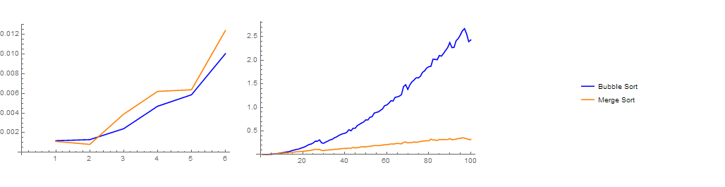
By comparing the plots of their running times, we can infer that, for **smaller** input sizes, both algorithm's have **similar** running times.
As the input size becomes **bigger** and bigger, both algorithm's running times increase but **bubble sort's running time increases noticeably faster**.
When it reaches sizes of around 100 elements, the difference between them is very obvious.
Merge sort algorithm becomes the clear winner in terms of running time.
### Measuring running time through instruction approximation
Another method of approximating the running time functions is by approximating the number of **instructions** executed during the algorithms lifetime[^5].
This method assumes that each instruction is executed in the same amount of time (1 arbitrary unit of time).
It also disregards all other extra factors that affect the running time besides the input size.
Using this method, I approximated the following runtimes for the code that I wrote.
- Bubble Sort: $T(n) = 4n^2 + 3$
- Merge Sort: $T(n) = 6n \log_2 {n} + 5n + 2$
[^5]:
Don't worry about the how I ended up with these functions.
For now just accept that these are the running times I ended up with.
You'll tackle this topic on CMSC 142
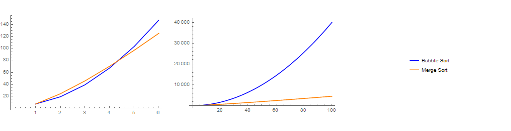
The running time functions that we ended up with also shows that for **smaller input sizes** both algorithms end up executing pretty much the same amount of instructions.
For **larger input sizes**, it also shows that merge sort is clear winner, it ends up executing way fewer instructions compared to bubble sort.
For both of these methods we end up with similar conclusions.
**Merge sort is the preferred algorithm between the two**.
Even though, bubble sort may be faster than merge sort for smaller input sizes, **for cases that matter the most (large input sizes), merge sort is way faster**.
When we use these algorithms in the real setting, we will be most concerned about how these algorithms perform on large input sizes.
That's because **we expect that larger input sizes will take a longer time** to compute for.
Because of this we barely care about how the algorithms compare for smaller input sizes, **we instead focus on the bigger picture that matters most**.
**Which algorithm performs better in stressful situations (when the input sizes go big).**
But here's the problem with what we are doing so far.
What we are comparing in these two representations (experimental running time and approximate instruction running time) are running times for the **written code** for the algorithms, not the algorithm's themselves.
These running time measurements are attributed specifically to the Python **code** I wrote for the algorithm.
What happens if the I wrote the code in a different language? What happens if I run it in a different processor?
### Finally, Asymptotic Notation
So what does all of this tell us?
1. **Algorithm efficiency is highly dependent on input size, the best representations of efficiency is a function.**
2. **There is no reliable way to compare algorithm efficiency.
The ways that we have always end up being approximations.**
3. **We care the most about how the algorithm performs in large input sizes**
All of these factors reveal to us that the best way to compare algorithms is by the use of asymptotic notation.
1. **Since algorithm efficiency almost always ends up being functions of input sizes, we can makes use of asymptotic notation, which compare relationships between functions.** Remember that the member's of O, $\Omega$, $\Theta$, o, $\omega$, are functions.
We've even shown how asymptotic relationships are similar to inequality/equality relationships, but instead of comparing numerical values, we compare functions.
2. **You'll find that asymptotic notation relationships are good at calculating approximated values.** The asymptotic relationships between two functions still hold true even if you change the functions a little bit.
For example $2n^2 + 5n \in \Theta(4n^2+3)$, even if we change the constant coefficients in these functions, their asymptotic relationship still stays the same: $an^2 +bn \in \Theta(cn^2 + d)$.
This characteristic is useful in the case of running time comparisons because as we've shown, our methods of measurements are not precise enough or uniform enough.
Asymptotic notation doesn't care about the small mistakes in measurement.
3. **Asymptotic notation by definition only cares about large values of $n$.** If we recall, asymptotic relationships only care about what happens on **sufficiently large values of $n$**, or on values of $n\to \infty$.
So to apply asymptotic notation to merge sort and bubble sort, we can use the functions we got by measuring the instructions in python code.
We can conclude that:
$$
4n^2 + 3 \in \Omega(6n \log_2 {n} + 5n + 2)
$$
This leads us to the conclusion that bubble sort's **time complexity** is higher than merge sort's time complexity.
Time complexity of an algorithm is the conceptual asymptotic relationship ranking of an algorithm.
The lower the algorithm's time complexity is, the faster it performs on large input sizes.
Time complexity can also refer to how fast the algorithm's running time increases as the input size increases.
An algorithm with lower time complexity, is more efficient.
## Reduction Rules and Complexity Classes
I've mentioned it briefly in the previous section.
One of the things that make asymptotic notation a good benchmark for algorithm efficiency is its usefulness in calculating approximated value.
This is because asymptotic notation is only interested in comparing the function values on large values of $n$.
For example in a function such as $2n^2 + 5n$, In extremely large values of $n$ the term $2n^2$ will be contributing way more in the overall sum compared to the term $5n$.
This contribution will in fact be so large that we can ignore the influence of term $5n$ and the complexity of their sum will still be the same.
This is one of the characteristics of asymptotic notation that you'll learn, so that you can easily infer an algorithms time complexity.
Here are the other properties of asymptotic notation.
These properties helps us remove the unnecessary parts of a function without changing its complexity.
These are called reduction rules.
Applying these rules will strip a function down into its complexity class.
### Reduction Rules
#### Dropping the coefficient
$$
c>0 \to cf(n) \in \Theta(f(n))
$$
**Given a function multiplied to some constant, $cf(n)$, its complexity is exactly the same as $f(n)$.** This property can easily be demonstrated using the limit definition of $\Theta$.
##### Proof
$$
\lim_{n \to \infty}{\frac{cf(n)}{f(n)}}=\lim_{n \to \infty}{c}=c
$$
#### Higher degree polynomial
$$
c<d \to f(n)^c \in o(f(n)^d)
$$
**Given $f(n)^c$ and $f(n)^d$ where $c$ and $d$ are constants and $c<d$, $f(n)^c$ is less complex than $f(n)^d$**
##### Proof
$$
\begin{aligned}
\text{Let $0<c<d$}\\\\
\lim_{n \to \infty}{\frac{f(n)^c}{f(n)^d}}&=\lim_{n \to \infty}{\frac{cf(n)^{c-1}\frac{d}{d n}f(x)}{df(n)^{d-1}\frac{d}{d n}f(x)}}\\
&=\lim_{n \to \infty}{\frac{cf(n)^{c-1}}{df(n)^{d-1}}}\\
&=\lim_{n \to \infty}{\frac{c(c-1)f(n)^{c-2}}{d(d-1)f(n)^{d-2}}}\\
&\vdots\\
&=\lim_{n \to \infty}{\frac{c(c-1)(c-2)(c-3)\cdots(c-(c-1))f(n)^{c-c}}{d(d-1)(d-2)(d-3)\cdots(d-(c-1))f(n)^{d-c}}}\\
&=\lim_{n \to \infty}{\frac{c(c-1)(c-2)(c-3)\cdots(c-(c-1))}{d(d-1)(d-2)(d-3)\cdots(d-(c-1))f(n)^{d-c}}}\\
\lim_{n \to \infty}{\frac{f(n)^c}{f(n)^d}}&=0
\end{aligned}
$$
#### Sum of functions
$$
f(n) \in \Omega(g(n)) \to f(n)+g(n)\in \Theta(f(n))
$$
**In a sum of functions, the most complex function dominates the sum therefore the overall complexity will be equal to the dominant function.** This can be shown using the set definitions.
##### Proof
$$
\begin{aligned}
\text{Since} f(n) &= \Omega(f(n)),\\\\
\text{for any $n>n_0$}\\\\
f(n)&\geq cf(n) \\
f(n) +g(n)&\geq cf(n)
\end{aligned}
$$
Adding $g(n)$ to the left hand side of the inequality does not change the inequality relationship since $g(n)$ is positive (meaning, adding $g(n)$ can only result to increasing the value of the already bigger value). Therefore,
$$
\therefore f(n)+g(n)=\Omega(f(n))
$$
We can also show that $f(n) + g(n) \in O(f(n))$,
$$
\begin{aligned}
\text{Since } g(n) &= O(f(n)),\\\\
g(n)&\leq cf(n) \\
f(n)+g(n)&\leq cf(n) + f(n)\\
f(n)+g(n)&\leq (c+1)f(n)\\
\end{aligned}
$$
Therefore,
$$
\therefore f(n)+g(n) \in O(f(n))
$$
Since the sum $f(n) + g(n)$ is both $\Omega(f(n))$ and $O(f(n))$
$$
\begin{aligned}
& f(n)+g(n)=\Omega(f(n))\\
\land & \underline{f(n) + g(n) \in O(f(n)) \to}\\
& f(n)+g(n) \in \Theta(f(n))
\end{aligned}
$$
#### Different bases on log
**Bases for logarithms doesn't matter in terms of asymptotic notation therefore $\log_b{n}$ for any base is of complexity $\Theta(\log n)$.** Because of this we can omit the base of the logarithm since its value is irrelevant from the complexity.
##### Proof
$$
\begin{aligned}
\lim_{n \to \infty} {\frac{\log_a{n}}{\log_b{n}}}&=\lim_{n \to \infty} {\frac{\frac{\log_b{n}}{\log_b{a}}}{\log_b{n}}}\\
&=\lim_{n \to \infty} {\frac{\log_b{n}}{\log_b{n}(\log_b{a})}}\\
&=\lim_{n \to \infty} {\frac{1}{\log_b{a}}}\\
\lim_{n \to \infty} {\frac{\log_a{n}}{\log_b{n}}}&=\frac{1}{\log_b{a}}
\end{aligned}
$$
#### Different bases on exponential functions
$$
0<a<b \to a^n \in o(b^n)
$$
**Bases for exponential functions on the other hand matter**, as shown in this proof:
##### Proof
$$
\begin{aligned}
\lim_{x \to \infty}{\frac{a^n}{b^n}}&=\lim_{x \to \infty}{\frac{a^n}{(a^{\log_{a}b})^n}}\\
&=\lim_{x \to \infty}{\frac{a^n}{(a^n)^{\log_{a}b}}}\\
&=\lim_{x \to \infty}{(a^n)^{1-\log_{a}b}}\\
\end{aligned}
$$
Since $b>a$, then, $1-\log_a b<0$.
Therefore,
$$
\lim_{x \to \infty}{\frac{a^n}{b^n}}=0
$$
Based on these rules a complicated looking function can be **reduced** to the **simplest function** that matches its complexity.
For example, In the function below, the we can look for the most complex term in this sum and drop the rest.
In this case the term $6n \log_2 {n}$ is the most complex, so we apply the first sum of functions rule and drop the rest.
$$
6n \log_2 {n} + 5n + 2 \in \Theta(6n \log_2{n})
$$
After this we can apply the coefficient rule and drop the coefficient:
$$
6n \log_2 {n} + 5n + 2\in \Theta(n \log_2{n})
$$
And then apply the logarithm bases rule and drop the base since bases don't matter as well:
$$
6n \log_2 {n} + 5n + 2\in \Theta(n \log{n})
$$
This tells us that the complexity of $6n \log_2 {n} + 5n + 2$, is the same as $n \log{n}$.
By finding this out, **we can use $n \log n$ as sort of the representative of $6n \log_2 {n} + 5n + 2$ on matters regarding its complexity**.
### Complexity Classes
This reduction process is something that computer scientists do a lot.
When we compare algorithms, we compare them using these simple looking functions that represent their time complexity.
In the domain of computer science we know a few of these _representative_ functions, we call these, **complexity classes**.
One of the skills you will master as you mature as computer scientists is to be able to automatically identify any algorithm's complexity class.
By knowing an algorithm's complexity class we can easily infer how the algorithm will perform.
Here are the complexity classes in computer science, arranged from least complex, to then most complex
| Complexity Class | Name | Example |
| --------------------------- | ---------------- | --------------------------------------- |
| $\Theta(1)$ | Constant | converting Celsius to Fahrenheit |
| $\Theta(\log n)$ | Logarithmic | binary search |
| $\Theta((\log n)^c)$ | Polylogarithmic | dynamic planarity testing of a graph |
| $\Theta(n^c)$ where $0<c<1$ | Fractional power | primality test |
| $\Theta(n)$ | Linear | finding the smallest number in an array |
| $\Theta(n \log{n})$ | Quasilinear | merge sort |
| $\Theta(n^2)$ | Quadratic | bubble sort |
| $\Theta(n^c)$ where $c > 1$ | Polynomial | naïve matrix multiplication |
| $\Theta(c^n)$ | Exponential | dynamic travelling salesman |
| $\Theta(n!)$ | Factorial | brute force travelling salesman |
### Using O versus using $\Theta$
When specifying time complexity, you'll find that it is usually expressed in terms of **O**.
You might find this strange since **expressing the time complexity in terms of $\Theta$ is more specific**.
If someone says that an algorithm is $O(n^2)$ for example, the person is saying that the algorithm is at most as complex as $n^2$.
Were not sure if the exact complexity is indeed $\Theta(n^2)$, or $\Theta(n)$, or $\Theta(n \log n)$.
If you want to be as specific as possible, use, $\Theta$ to express complexity.
But sometimes the time complexity of an algorithm may be dependent on factors other than input size.
One of these factors for example is how the input is configured.
In the context of sorting, this will refer to the initial sortedness of the array.
Some algorithms perform under different time complexities depending on the initial conditions.
When an algorithm's complexity is expressed as some $O(f(n))$, this will tell you that, at its worst possible case, (for example in quick sort the worst case could be reverse sorted) the algorithm runs at $O(f(n))$, but there is still a possibility that on other cases, the algorithm will perform $o(f(n))$ (better than $f(n)$).
You'll find that **computer scientists will end up expressing time complexities in terms of $O$ as well because we generally want our algorithms to run on some acceptable standard of complexity**.
Because of this **asymptotic notation in terms of $O$ will usually suffice**.
 Sign in with Wallet
Connect another wallet
Sign in with Wallet
Connect another wallet