---
date: 1 April 2020
category: CMSC57
description: A lot of structures in mathematics and computer science can be characterized by complex connections and relationships. These structures are intimately known to computer scientists as graphs and trees.
---

# Graphs and Trees

A lot of structures in mathematics and computer science can be characterized by complex connections and relationships. These structures are intimately known to computer scientists as graphs and trees.

# Graphs

A **graph** commonly denoted as $G=(V,E)$, where $V$ is a nonempty set of **vertices** (sometimes called **nodes**) and $E$ is a set of **edges**. Each edge connects two vertices in $V$.

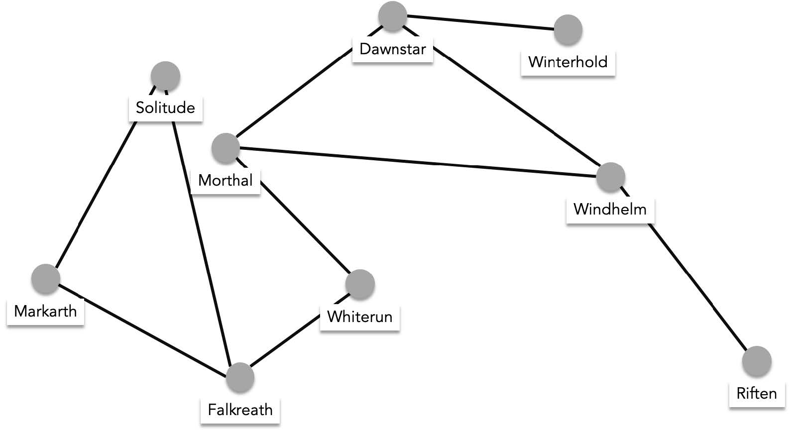
An example is a transportation network that is represents cities as vertices and roads as edges:

$V$={"Whiterun", "Falkreath","Solitude", "Markarth", "Morthal", "Dawnstar", "Winterhold", "Windhelm", "Riften"}

$E$={{"Whiterun", "Falkreath"}, {"Whiterun", "Morthal"}, {"Falkreath","Markarth"}, {"Falkreath", "Solitude"}, {"Morthal", "Windhelm"}, {"Morthal", "Dawnstar"}, {"Dawnstar", "Winterhold"}, {"Windhelm", "Riften"}}

To visualize this graph we draw labelled dots as vertices and connect dots if an edge exists between them:


> Note that the exact location of the dots are not part of the characteristics of the graph, The dots can be arbitrarily placed anywhere.

## Directed and Undirected Graphs

The example shown above is called an undirected graph. An undirected graph means that if any two vertices $a$ and $b$ are connected, $b$ and $a$ are also connected. Meaning the connection between $a$ and $b$ goes both ways. Formally an undirected graph $G=(V,E)$ is a graph defined such that, $\forall a\in V,b\in V(\{a,b\}\in E \to \{b,a\} \in E)$. Simply put, if a graph is specified to be undirected $\{a,b\} \in E$ automatically means $\{b,a\}\in E$.

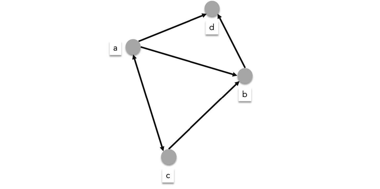
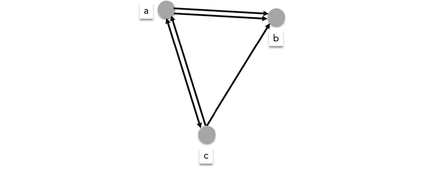
A directed graph is a generalization where the direction of the connection between two vertices matter. $(a,b)\in E$ Does not necessarily mean $(b,a)\in E$. When visualized a directed graph's edges are drawn as arrow to specify the direction:


> An undirected graph's edge is denoted using unordered pair, (note the curly braces"{ }") while a directed graph's edge is denoted using an ordered pair, (note the parenthesis).

## Simple graphs and multigraphs

The graphs we have looked at so far are examples of **simple graphs**. Simple graphs are graphs where there are at most 1 edge for every pair of vertex. If at least one pair of vertex has more than one edge then that graph is a **multigraph**. The graph below is an undirected multigraph since there are two of $\{a, c\}$ and two of $\{b,c\}$.


The graph below is a directed multigraph since there are two of $(a,b)$ and two of $(c,a)$.


## Some important graph terminologies

- **adjacency** - vertices $a$ and $b$ are said to be **adjacent** or **neighbors** in $G$ if $(a,b)\in E$. We also say $(a,b)$ **connects** $a$ to $b$ or $e$ is **incident with** $a$ and $b$.
- **neighborhood** - the neighborhood of some vertex $a$ in graph $G(V,E)$, usually denoted as $N(a)$, is the set of all neighbors of $a$ in $G$. Given some set of vertices $A$, $N(A)$ is the set of vertices that are neighbors of at least one vertex in $A$.

- **degree** - the degree of a vertex in an undirected graph, denoted by $\deg(a)$ is the number of edges that connect to $a$. In an undirected graph $\{a,b\}$ and $\{b,a\}$ are counted as one degree. In the example below, $\deg(\text{"Morthal"})=3$, $\deg(\text{"Whiterun"})=2$


> **Loops and degrees** - Some graphs contain special edges called loops. Loops are edges where the endpoints is one vertex. In the example below one of the edges is an edge that connects $a$ to itself, $(a,a)$.
>
> 
>
> It is important to note that when counting the degree of $a$, the loop, $\{a,a\}$ is counted twice. Therefore, $\deg(a)=3$. This might seem strange but there are a couple of reasons why graph theorists decided to define it as such. One of the reasons is the following: if you look at a non-loop edge, like $\{a,b\}$, this edge is counted as the edge of $b$ and counted as an edge of $a$ again. Meaning, in the total degree of the graph, $\{a,b\}$ is counted exactly **twice**. Applying the same reasoning to a loop like $\{a,a\}$, means that this edge must be counted once for vertex $a$ and another for the other vertex $a$. Meaning it must be counted twice as well.

- **degree sum** - the sum of all degrees of all vertices in some graph $G=(V,E)$ is exactly twice the number of edges. This is known as the **handshaking theorem** which formally states that $\sum_{v\in V}{\deg(v)}=2|E|$. This is again because each edge is counted twice as a degree, one for each vertex it connects.

## Some special graphs

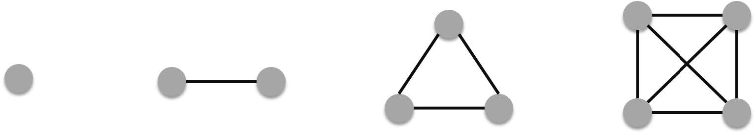
### Complete graphs

Complete graphs are graphs where any combination of two vertices are connected by an edge. This means that a complete graph with $m$ edges contain the maximum amount of edges. Graphs that are not complete are incomplete graphs.


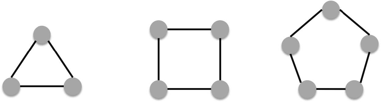
###### Cycles

Cycles are graphs with 3 or more vertices with the following edge pattern:

$E=\{\{v_1,v_2\},\{v_2,v_3\},\{v_3,v_4\},\cdots,\{v_n-1,v_n\},\{v_n,v_1\}\}$.


### Bipartite graphs

Bipartite graphs are special graphs where the vertices of the graph can be divided into two disjoint subsets such that each vertex of one subset is connected by an edge to one of the vertices in the other subset and vice versa. Also there must be no edge that connects vertices from the same subset. This means that in a bipartite graph all edges connect one from each vertex subset. Bipartite graphs are important for modelling matching problems and pairwise association problems.

For example, a cycle of 6 vertices is bipartite as shown below:


## Graphs Representations

When encountering graph related problems, you often need to devise a way to represent the graph into a convenient data structure. By representing graphs using these data structures you are able to solve problems such as connectivity, shortest paths, and etc.

### Adjacency list

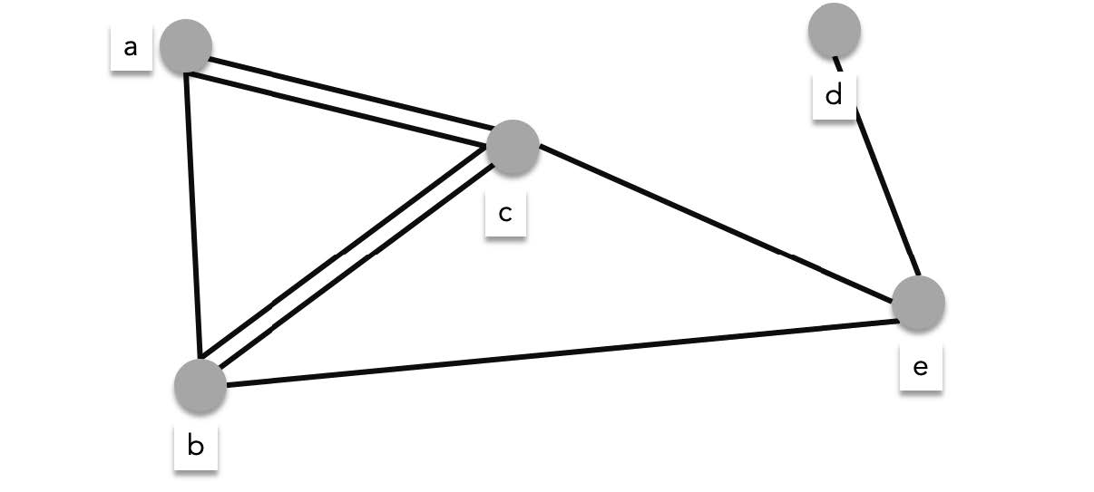
There are two main ways to do this, one is to list all vertices. For each vertex, list all the neighbors of the vertex. This method is called **adjacency list**. For example the graph below:


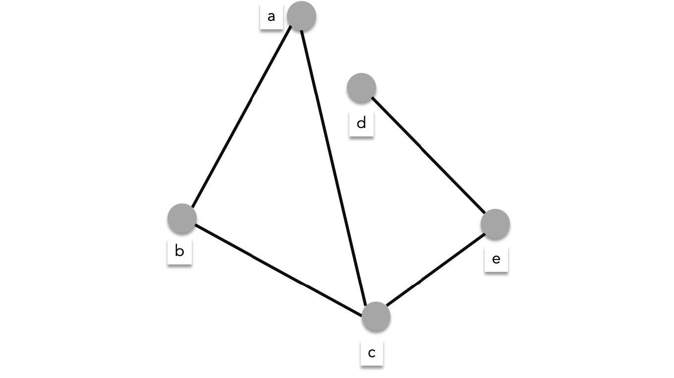
can be represented by the following adjacency list:

| vertex | neighbors |
| :----: | :-------: |
| a | b,c |
| b | a, c |
| c | a, b, e |
| d | e |
| e | c, d |

When representing a directed graph, only the **terminal neighbors** are listed. The terminal neighbors of an edge are the neighbors on the arrowhead of the edge. For example the following directed graph,


can be represented by the following adjacency list:

| vertex | terminal neighbors |
| :----: | :----------------: |
| a | b, c, d |
| b | d |
| c | a, b |
| d | *none* |

For multigraphs, when there are $n$ edges connecting two vertices, list the neighbor $n$ times. For example the multigraph below


| vertex | neighbors |
| :----: | :-------: |
| a | b, b, c |
| b | *none* |
| c | a, a, b |

### Adjacency matrix

Another way to represent the graph is to use an **adjacency matrix**. Given a graph with $m$ vertices, create an $m \times m$ matrix called $A$. Each vertex in the graph is associated to a number from $1$ to $m$, such that vertex $v_i$ is associated to the number $i$. If an edge connecting $v_i$ to $v_j$ exists, then the cell value at $A_{i,j}=1$. For example the same undirected graph,


can be represented by the following adjacency matrix:
$$
\begin{aligned}
&v_1=a,v_2=b,v_3=c,v_4=d,v_5=e\\\\
&A=\begin{bmatrix}
0 & 1 & 1 & 0 & 0\\
1 & 0 & 1 & 0 & 0\\
1 & 1 & 0 & 0 & 1\\
0 & 0 & 0 & 0 & 1\\
0 & 0 & 1 & 1 & 0\\
\end{bmatrix}
\end{aligned}
$$

> Notice that the adjacency matrix of an undirected graph is symmetrical ($A^T=A$). That is because, $A_{ij}=A_{ji}$ (i.e. edge $\{v_i,v_j\}$ exist if and only if $\{v_j,v_i\}$ exists).

For undirected graphs, $A_{ij}=1$ if and only if $(v_i,v_j)$ is an edge (i.e. $v_j$ is a terminal vertex connecting $v_i$). Therefore, the same directed graph,


can be represented by the following adjacency matrix:
$$
\begin{aligned}
&v_1=a,v_2=b,v_3=c,v_4=d\\\\
&A=\begin{bmatrix}
0 & 1 & 1 & 1\\
0 & 0 & 0 & 1\\
1 & 1 & 0 & 0\\
0 & 0 & 0 & 0\\
\end{bmatrix}
\end{aligned}
$$
For multigraph, when there are $n$ edges connecting two vertices $v_i$ and $v_j$, $A_{i,j}=n$,

$$
\begin{aligned}
&v_1=a,v_2=b,v_3=c\\\\
&A=\begin{bmatrix}
0 & 2 & 1\\
0 & 0 & 0\\
2 & 1 & 0\\
\end{bmatrix}
\end{aligned}
$$

## Paths and Circuits

A **path** along a graph, is a sequence of edges $(v_0,v_1),(v_1,v_2),\cdots ,(v_{n-1},v_n)$. A path describes a traversal from $v_0$ to $v_n$ along the edges of the graph. If the starting point and end point of a path with length greater than zero is the same edge, or $v_0 = v_n$, then that path is a **circuit**.

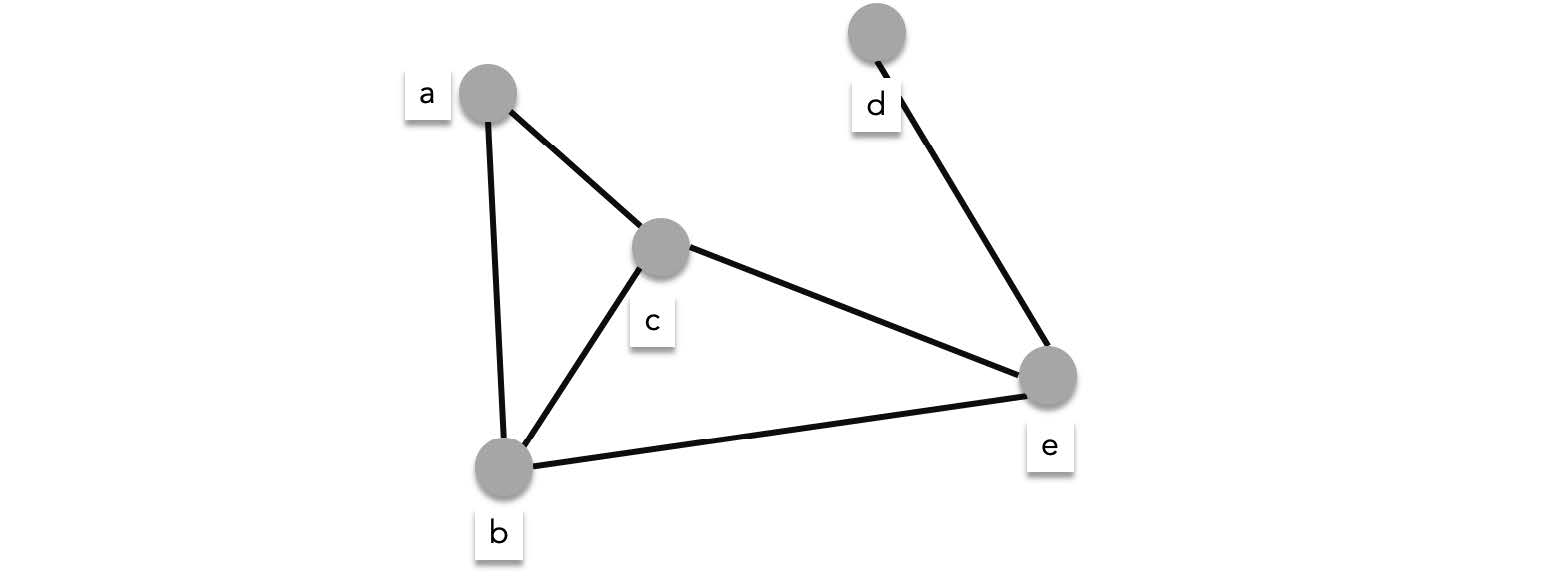
Given a graph $G$, if there exists a path connecting every distinct pair of vertices, then $G$ is **connected**.

The graph below is connected


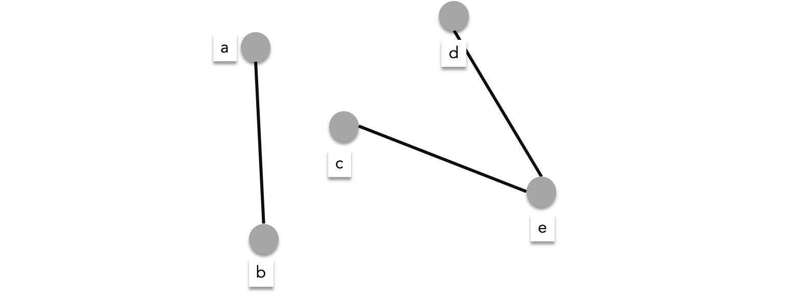
while the graph below is unconnected, since there is no path from $a$ to $c$, $d$, or, $e$ (there is also no path from $b$ to $c$, $d$, or, $e$)


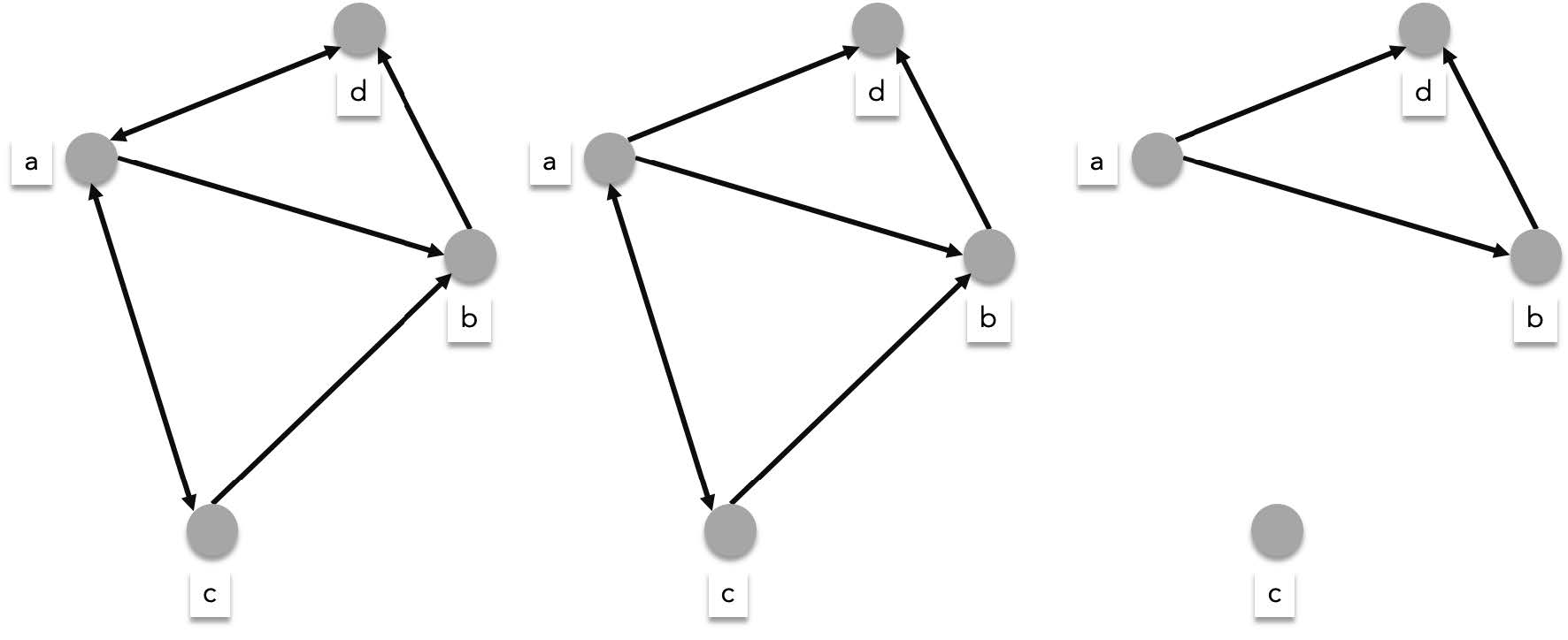
> For directed graphs, connectivity can either be strong or weak. A directed graph is **strongly connected** if there exists a path connecting every distict pair of vertices. A directed graph is **weakly connected** if it is not strongly connected but its couterpart undirected graph (i.e. the same directed graph except all edges are replaced with undirected edges) is connected.
>
> The leftmost graph is strongly connected. The middle graph is weakly connected (there is no path from $d$ to $a$, $b$, or $c$ but there will be if you the replace edges with undirected ones). The rightmost graph is unconnected.
>
> 

### Euler Circuits and Paths

One of the most well known graph theory related problems is the **seven bridges of Königsberg** problem. In the town of then Prussia called Königsberg, there were a total of seven bridges connecting 4 sections divided by the Pregel river. The townspeople of Königsberg wondered if there was a way to start at some section of the town, travel across all the bridges exactly once and return to the starting point. Leonhard Euler interpreted the problem as a graph problem (dated in 1736 arguably one of the first use of graph theory), represented by the multigraph below:


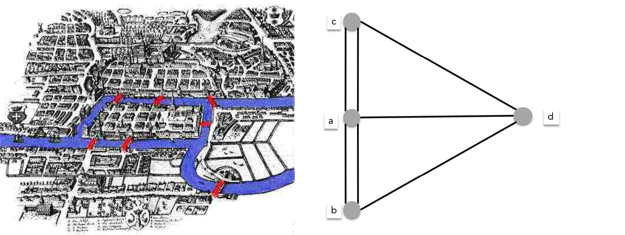
> Since bridges can be travelled on two directions, this is an undirected graph, one cannot travel from c to d and then d to c since you will travel on the same bridge twice.

As a graph problem, the seven bridges problem can be stated as the search for **a circuit containing all edges of the graph exactly once**. A circuit with these properties became known as an **Euler circuit**. On the other hand an **Euler path** is a path containing all edges of the graph exactly once.

While solving the seven bridges of Königsberg problem Euler was able to characterize the exact conditions for a graph for an Euler circuit to exist. Consider the following graphs, the graphs below contain Euler circuits:


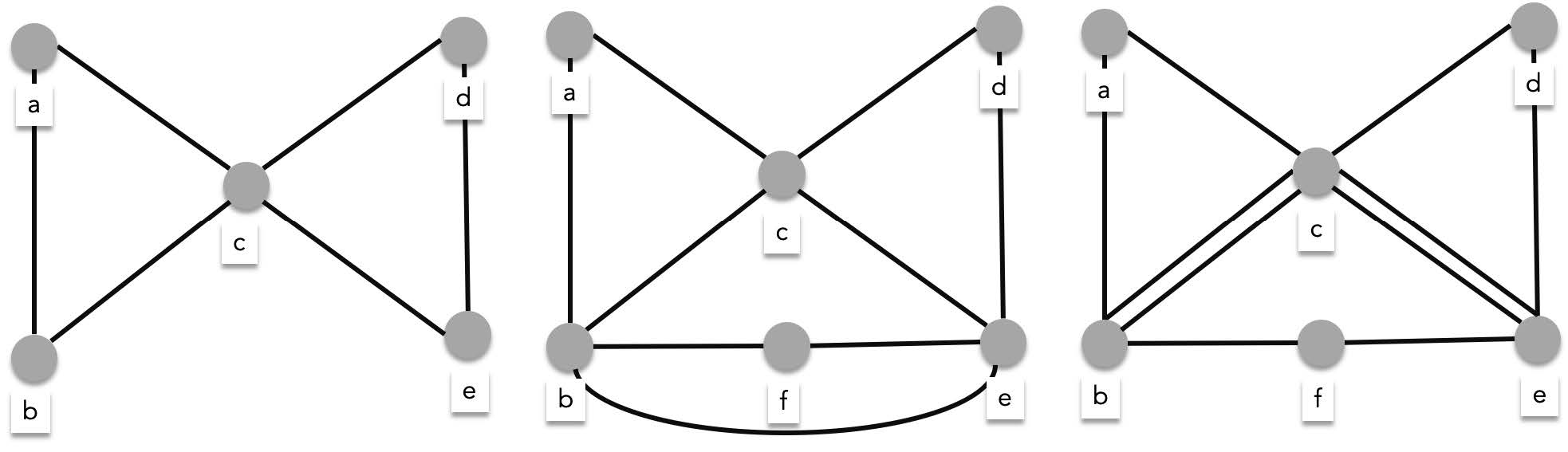
> - **leftmost graph** - $\{a, b\}, \{b, c\}, \{c, d\}, \{d, e\}, \{e, c\}, \{c, a\}$
> - **middle graph** -$ \{a, b\}, \{b, f\}, \{f, e\}, \{e, b\}, \{b, c\}, \{c, d\}, \{d, e\}, \{e, c\}, \{c, a\}$
> - **rightmost graph** -$ \{a, b\}, \{b, c\}_1, \{c, e\}_1, \{e, f\}, \{f, b\}, \{b, c\}_2, \{c, d\}, \{d, e\}, \{e, c\}_2, \{c, a\}$

While the graphs below do not contain Euler circuits:


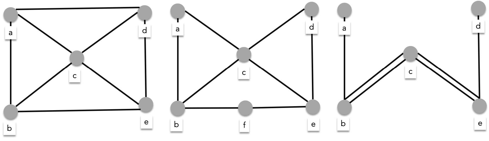
You'll notice that all the vertices of the graphs with Euler circuits have even degrees while some of the vertices of the graph with no Euler circuits have odd degrees. In fact this is what Leonhard Euler discovered when studying the seven bridges problem. A graph has an Euler circuit if and only if all its vertices have even degrees. We can prove this using the algorithm for searching an Euler circuit.

> **Proof**
>
> Given a connected multigraph $G = (V,E)$, where $\forall v \in V \exists k\in \mathbb{Z}(\deg(v)=2k)$ (i.e. all the vertices have even degrees). Starting from an arbitrary vertex $v_0$ we construct an Euler circuit, The first edge visited is $\{v_0, v_i\}$, by traversing this edge we exit $v_0$, leaving an odd number of untraversed edges connected to $v_0$ (thats because any even number minus one is odd). There are also an odd number of untraversed edges connected to $v_i$ because we have already traversed one of the edges connected to $v_i$, which is $\{v_0, v_i\}$.
>
> We are now currently at $v_i$. Leaving $v_i$ we traverse $\{v_i,v_j\}$, entering $v_j$. After leaving $v_i$, there is an even number of untraversed edges connecting $v_i$ (because odd minus 1 is even). Notice that after entering and exiting a vertex, we traverse exactly two edges from it, meaning that every time we pass through a vertex, (enter then leave) we leave an even amount of untraversed edges. Therefore, no matter how many times we enter a vertex, there will always be an edge to exit from.
>
> This proves that there cannot be an euler circuit for a graph with at least one vertex of an odd degree because you will get stuck in that vertex at some point. There will be no more edges left to exit from.
>
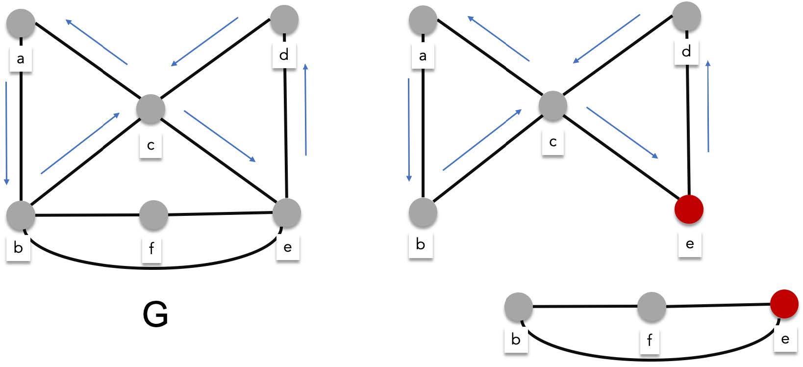
> After traversing an arbitrary amount of vertices, we will eventually return to $v_0$ thus creating a circuit. There are two possibilities when this happens, either we have successfully visited all edges, creating an actual Euler circuit, or we have not. If we have not successfully visited all the edges, you would at least have created an Euler circuit for the subgraph of the $G$. Lets call this subgraph $H$ and the subgraph left behind, I.
>
> 
>
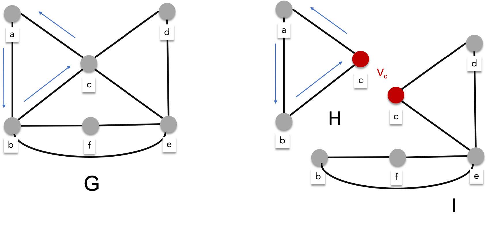
> Let the sequence of edges $Q=\{v_0,v_1\}, \{v_1,v_2\},\{v_2,v_3\}, \cdots, \{v_k,v_0\}$, be an euler circuit for the subgraph H. One of the properties of any circuit, is that you can rearrange the sequence starting anywhere, say $\{v_1,v_2\}$. If you transfer all the edges before $\{v_1,v_2\}$ to the end of the sequence, you will still have a circuit ($\{v_1,v_2\},\{v_2,v_3\}, \cdots, \{v_k,v_0\}, \{v_0,v_1\}$).
>
> Because of this you can start the traversal all over again but starting from a vertex that connects $H$ to $I$. Lets call this $v_c$. After traversing the euler circuit for $H$, you are now back to $v_c$. Continue the traversal from here and you'll either find the Euler circuit for entire graph $G$ or find the Euler circuit for a bigger subgraph. When that happens, you just redo the earlier steps until you find the complete Euler circuit.
>
> 

This shows that the seven bridges of Konigsberg do not have an Euler circuit.

### Hamilton circuits and paths

Hamilton circuits are similar Euler circuits. Instead of visiting every edge exactly once, you visit every vertex exactly once. A hamilton circuit can visit an edge either zero or one time.

Although these problems are similar and related, there is no known simple solution for finding Hamilton circuits (it is NP complete). There are some conditions that guarantee that a graph either has or has no Hamilton circuit. For example a complete and a cycle graph is guranteed to have a Hamilton circuit. A graph with a vertex of degree one is guranteed to not have a hamilton cycle

The example below shows a Hamilton circuit of a graph:


The graph below cannot have a hamilton cycle since $\deg(d) = 1$.


### Shortest path problems

Before we talk about shortest path problems, let us introduce weighted graphs. Weighted graphs are graphs where each edge has an associated value. For example the following graph's edges are associated to the distances between each connected vertex.


You might be interested to know the shortest distance between Windhelm and Morthal. Or you might be interested in finding the shortest path that visits every city in the map. Finding the shortest path that visits every vertex is also called the **travelling salesman problem**. Another well known difficult problem in CS.

#### Shortest path between two vertices

There are a lot of algorithms to find the shortest path between two vertices. What we will show is the well known Dijkstra's shortest path algorithm which searches the shortest path by greedily finding the shortest intermediate paths.

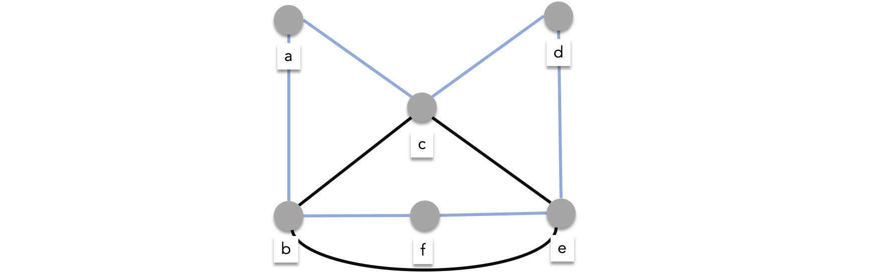
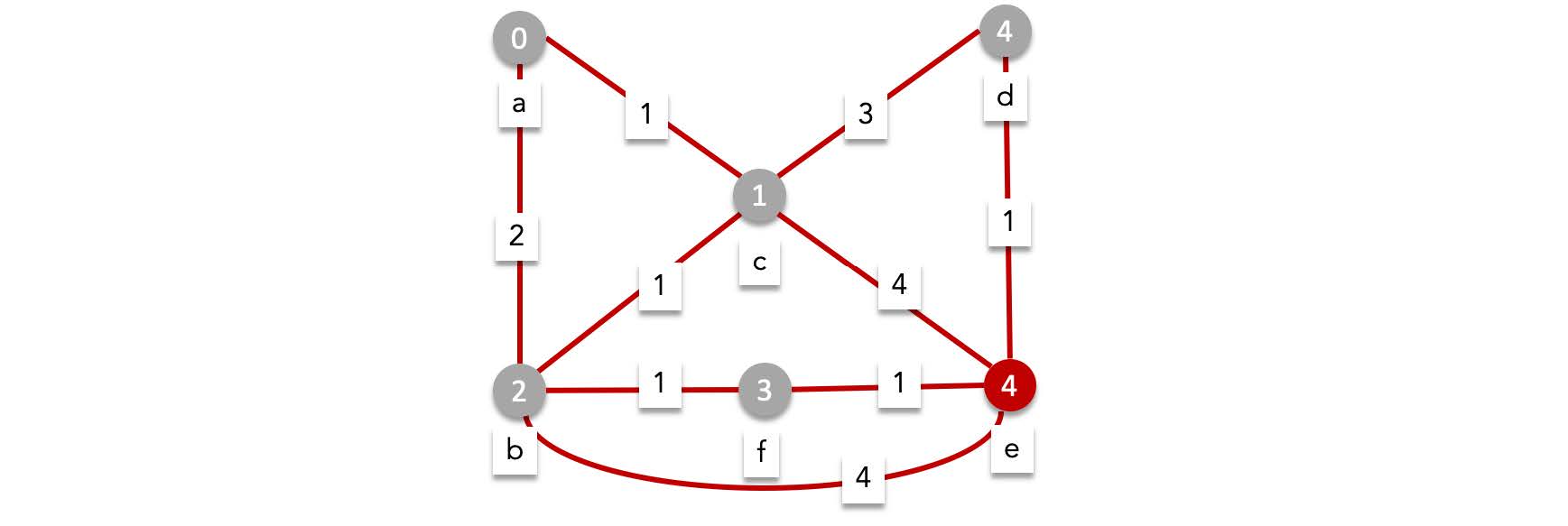
For example, consider the following graph. What is the length of the shortest path between $a$ and $e$?


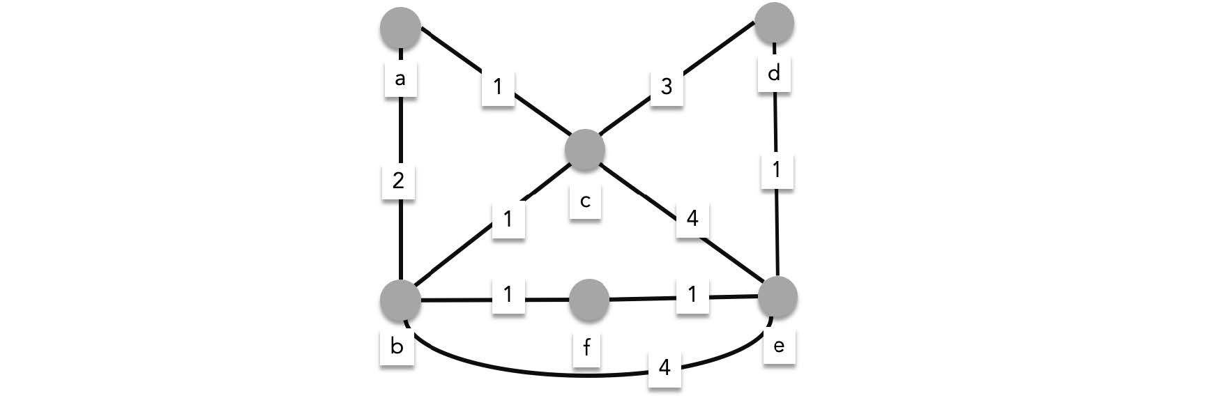
Starting from $a$, we have two choices, we can either traverse $\{a,c\}$, or $\{a,b\}$. These edges have lengths $1$ and $2$ respectively, meaning we are sure that the current shortest path to $c$ is $1$ and the current shortest path to $b$ is $2$. To avoid retraversing $\{a,c\}$ or $\{a,b\}$ we label these edges as visited. Retraversing these edges will only lengthen the path so we cannot traverse these edges ever again.


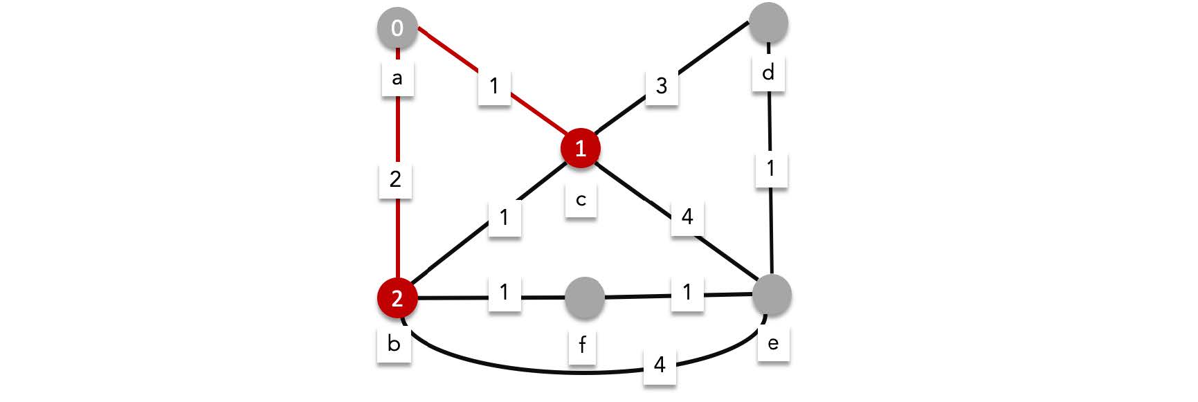
We continue the algorithm now while we are at $b$ and $c$. There are three edges from $b$ and three edges from $c$.

> The total path length to the next vertex is calculated by adding the shortest path until the current vertex plus the edge length to reach the next vertex. For example the total path to $f$ is shortest path to b plus length of $\{b,f\}$ (i.e. 2+1)

- From $b$ we can reach

- **$f$, with a total length of $3$,**
- $c$ with a total length of $3$,
- **$e$ with a total length of 6.**

We update the shortest paths for these vertices (except for $c$ since 1 is the current shortest path to reach it).

- From $c$ we can reach

- **$d$ with a total length of 4,**
- **$e$ with a total length of 5,**
- $b$ with a total length of $2$.

We update the shortest paths for these vertices replacing $e$ with 5, but not $b$ since the shortest path is currently $2$.

We then mark all the edges we traversed in this round as visited:


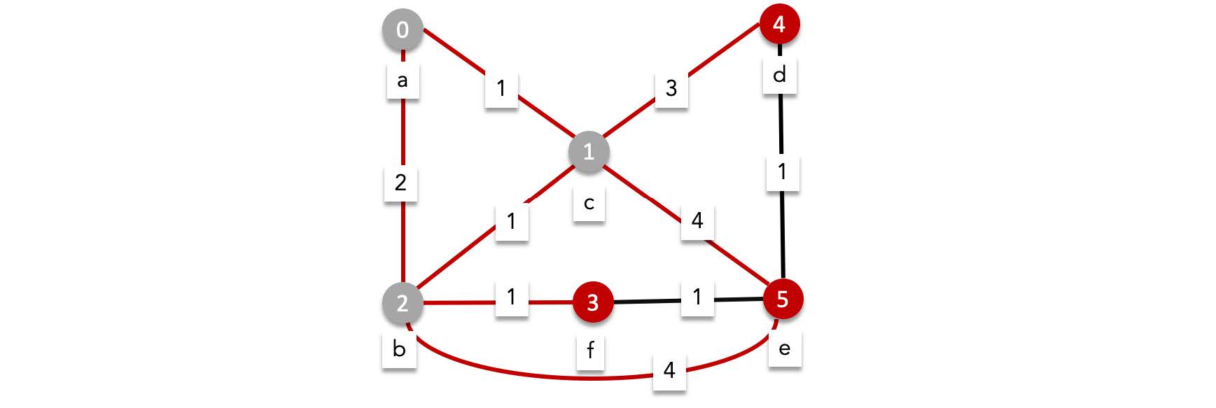
We are currently at the vertices $d$, $e$ and $f$. We can omit $e$ since it is our destination.

- From $d$ we can reach

- $e$ with a total length of $5$.

- From $f$ we can reach

- $e$ with a total length of $4$.

We update the shortest path to $e$ as $4$.

After this round we have visited all possible edges, concluding that the shortest path to $e$ has length $4$.


> To figure out the actual shortest path not just the length, you can record the path along with the length. You can also figure out the shortest path by backtracking from the destination vertex and figure out the previous vertex based on the edge lengths

#### Travelling Salesman Problem

The travelling salesman problem named after a situation where a salesman finds the most efficient way to travel across a map that visits all locations Usually there is an extra restriction where the salesman must return to the starting location. This can be rephrased into a graph problem as :

*finding the minimum length circuit that visits all vertices in the graph*

You'll notice that the travelling salesman problem is very similar to the hamilton cycle. In fact the solution to the travelling salesman problem is as complicated as the solution for hamilton cycles. In fact these problems are belong to a class of problems known as **NP-Complete** which are the most difficult among difficult problems in computer science.

> Note that there are solutions to these problems. It's just that the known solutions to these problems are algorithms that run in $\Omega(n^c)$.

# Trees

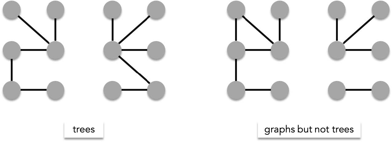
Trees are special graphs have the following characteristics

- **simple** - all of the edges are distinct
- **connected** - there exists a path between any two vertices
- **acyclic** - it contains no circuits that repeat edges ($\{v_i,v_j\}, \{v_j,v_i\}$ is technically a circuit but these can exists in trees)


Trees are useful mathematical structures that are usually used to characterize special relationships like hierarchy, recursive structures and composition. Computer file structures are example of recursive structures (folders can be composed of subfolders) that are represented using trees. A family tree which highlights a hierarchal structure are also represented by trees.

### Root

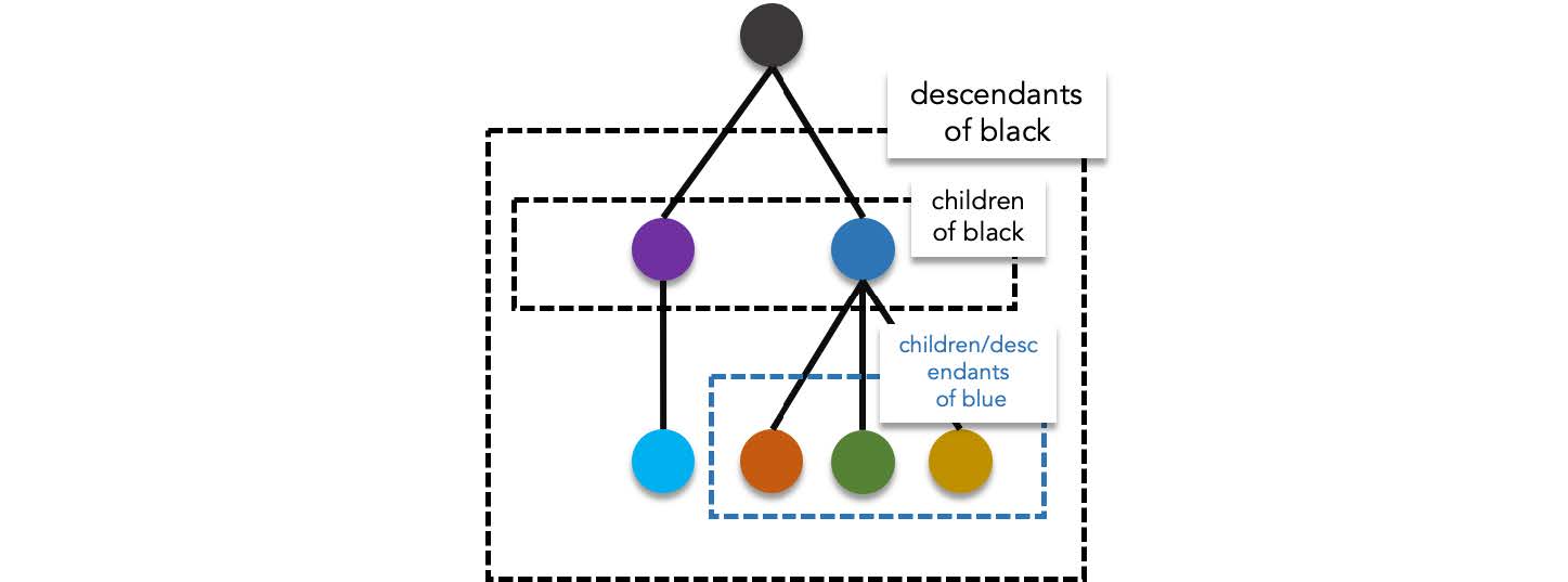
A tree is usually characterized with a special vertex designated as the origin for all paths in the tree. This vertex is known as the **root**. The root of a tree is important in hierarchal structures since it is where the "highest" vertex resides. By designating a root, a tree can be structured in a way where the relationship between a any two vertices that share an edge is that of a **parent** and **child**. The children of a vertex (also called a **subtree**) are the neighbors of said vertex found hierarchally below. The parent of a vertex (also called a **supertree**) is the sole neighbor found hierarchally above the vertex. The root is the only vertex that does not have a parent.

The **descendants** of a vertex includes, the children of said vertex, the children of the children of said vertex (also known as the grandchildren), the children of the children of the children of said vertex (also known as great grand children), and so on. The **ancestors** of a vertex are the opposite. It includes, the parent of a vertex, the parent of the parent of said vertex (also known as the grandparent), the parent of the parent of the parent of said vertex (also known as the great grand parent.), and so on. Vertices that share the same parent are known as **siblings**. A vertex without children is called a **leaf**.


> Descendants and ancestors can be described recursively:
>
> $u$ is descendant of $v$ if either:
>
> - $u$ is a child of $v$ or,
> - $u$ is the descendant of the child of $u$.
>
> $u$ is an ancestor of $v$ if either:
>
> - $u$ is the parent of $v$ or,
> - $u$ is the ancestor of the parent of $v$.

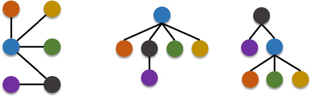
The designation of the root vertex is very important that changing the designated root of a tree changes the tree structure itself. For example the same graph below can be represented by more than one rooted tree. If the blue vertex is designated as root or if the black vertex is designated as root.


> When working with rooted trees, a vertex becomes some sort of representative for the vertices below it. For example in the tree below, when you refer to the tree $a$, you refer to the rooted tree formed by $a$ and its descendants:
>
> 
>
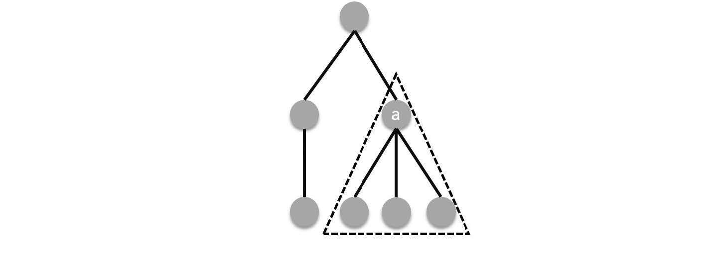
> This is what it means when we say that a tree is a recursive composite structure. A tree is either a leaf (which is also a tree) or composed of subtrees, which are also trees. Since these subtrees are also trees they can also either be trees or composed of subtrees.

### Tree Traversals

When characterizing rooted trees, it is important to devise a way to traverse all of the vertices in a specific order. Given a tree $T$, a traversal of $T$ is an ordered sequence of vertices.

#### Breadth First Traversal

Breadth first traversal starts at the root node and visits all nodes on the a level before visiting nodes in the lower level. Given two nodes $u$ and $v$, where $u$ is in an older generation than $v$, then $u$ will be visited first before $v$.

Traversing a tree breadth first uses a data structure called a queue. A queue is a list with only two actions, enqueue and dequeue. Enqueuing adds an item to the tail end of the list while dequeuing removes an item at the head of the list. Breadth first search works as follows:

Enqueue the root, while there are items in the queue, dequeue an item and enqueue every child of said item. Nodes are visited by order of dequeue.

For example, in the tree below, we start by enqueuing the root node $a$.


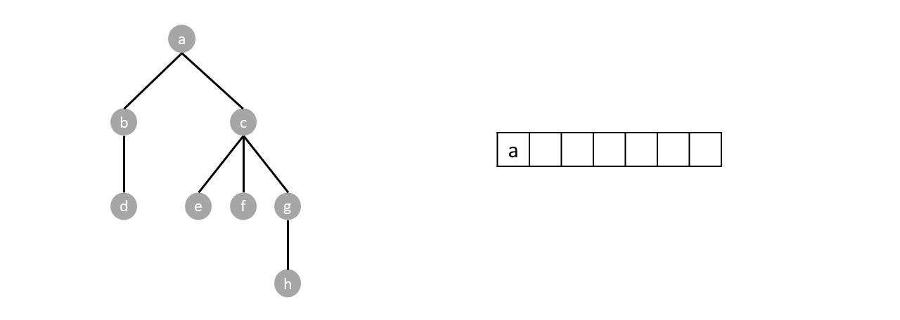
Since the queue is not empty we dequeue one item which happens to be $a$. We then enqueue every child of the dequeued item (node $a$), which are node $b$ and node $c$, as shown below: (the order of enqueuing children doesn't matter. Enqueuing $c$ then $b$ is still a valid breadth first traversal.)


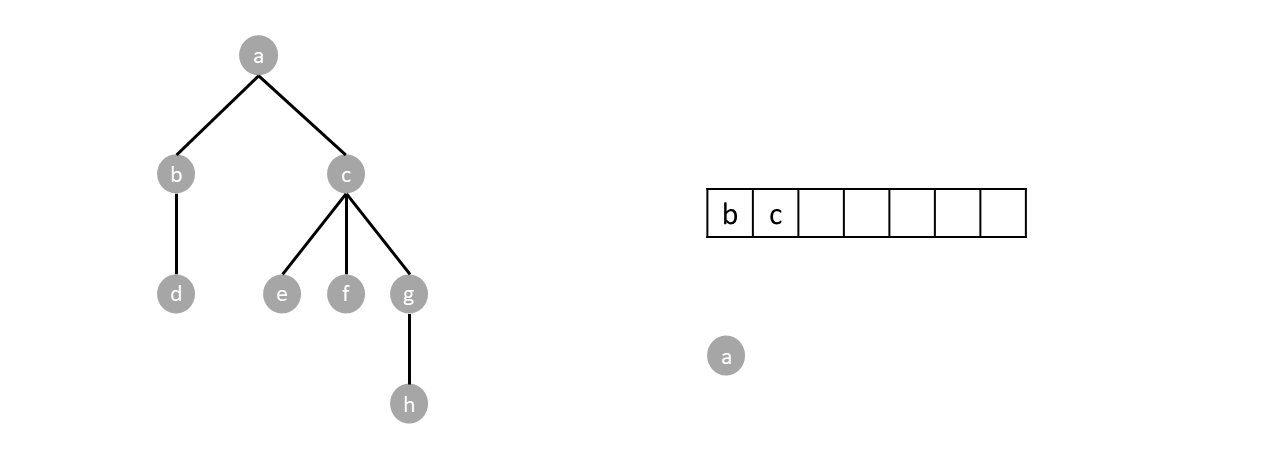
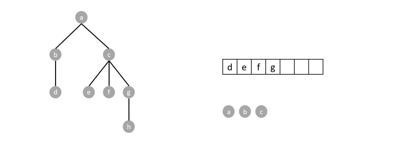
Since the queue is not empty we repeat the process by dequeuing one (node $b$), and enqueuing its children (node $d$).


We continue until the queue is empty completing the traversal.







#### Depth first traversal

Depth first traversal traverses a branch of a tree as far as possible before traversing other branches. Depth first traversal algorithm uses a stack instead of queue. It can also be represented as a recursive process.

A stack is a list with two actions, push and pop. Push adds an item at the head of the list while pop removes an item at the head of the list. The algorithm works as follows:

Push the root. While there are items in the stack, pop an item and push every child of said item. Nodes are visited by order of pops.

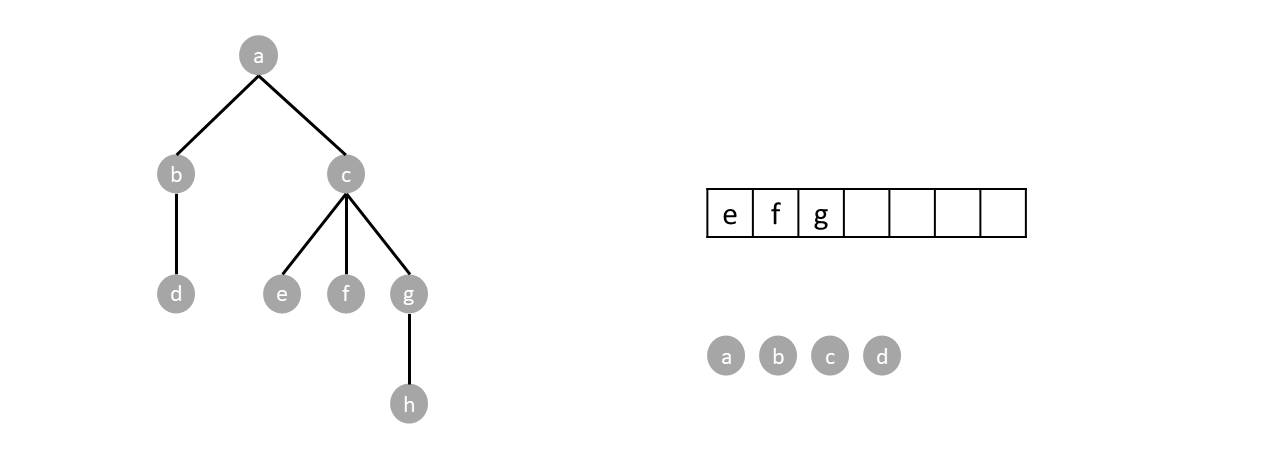
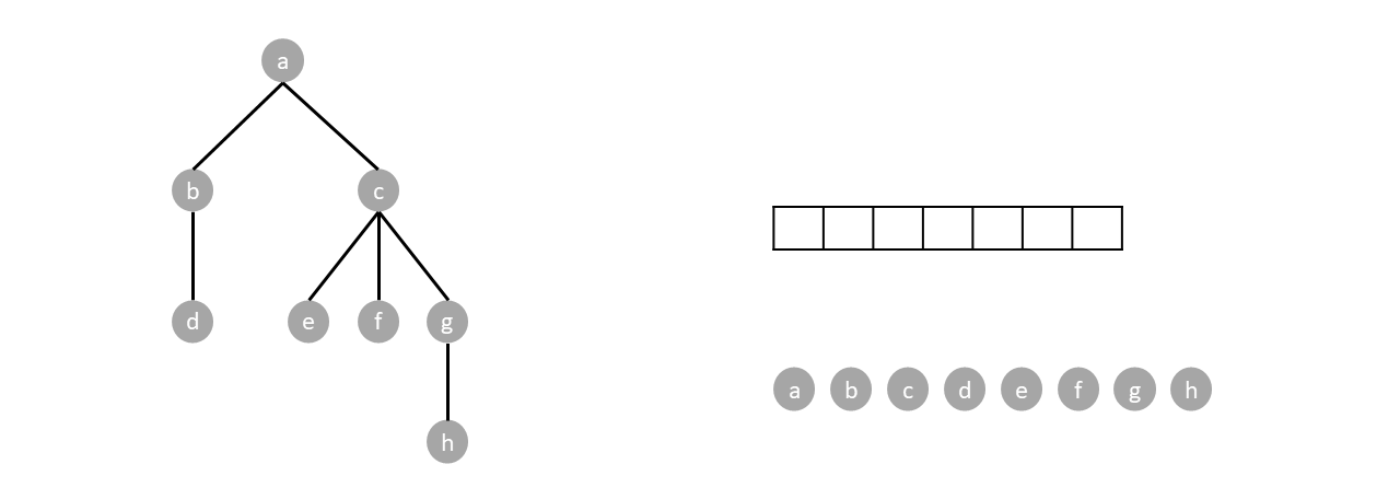
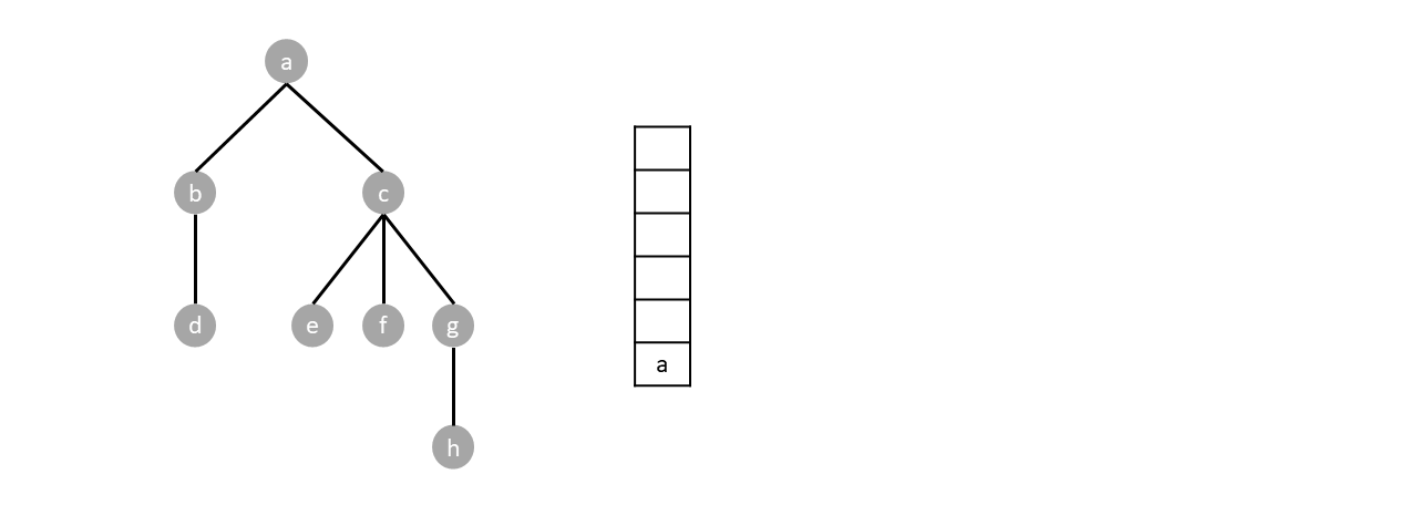
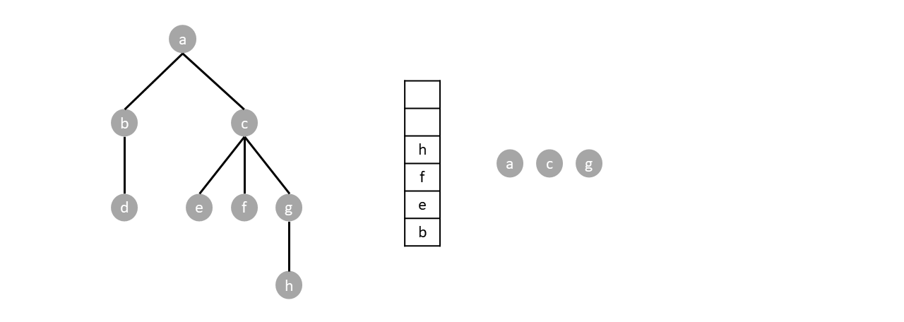
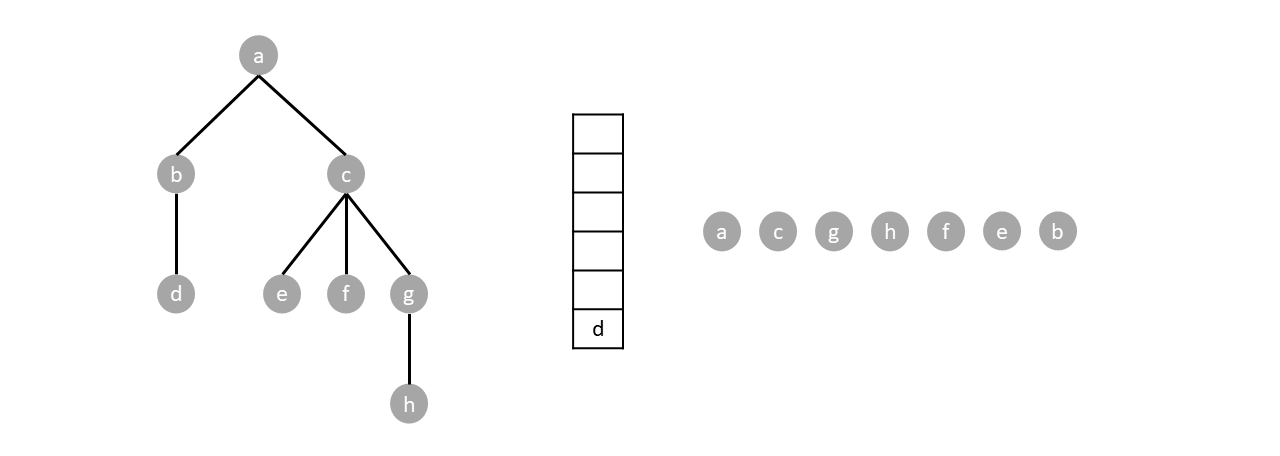
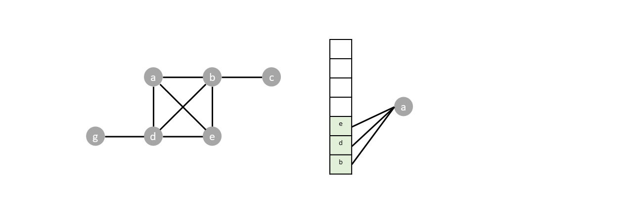
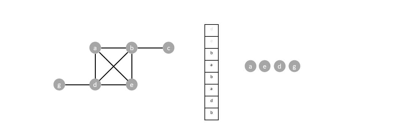
For example. In the tree below, we start by pushing the root $a$.


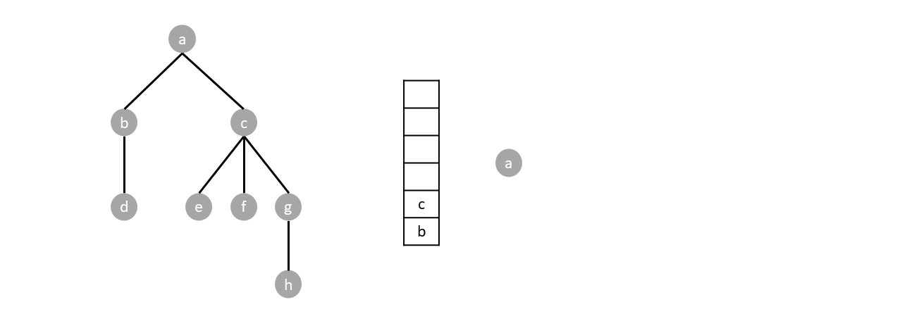
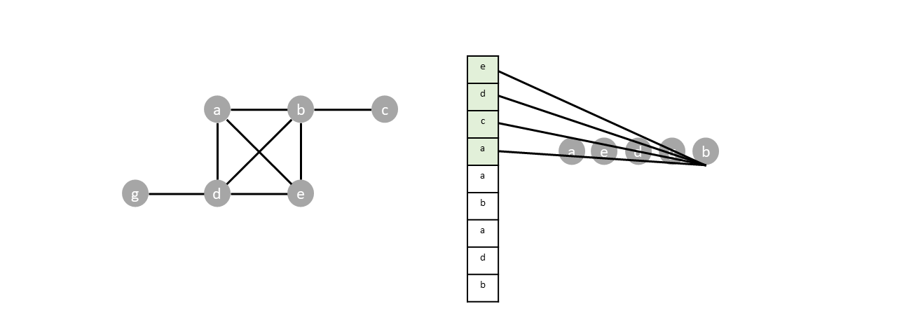
Since the stack is not empty we pop one item (node $a$) and push said items children.


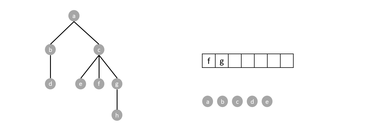
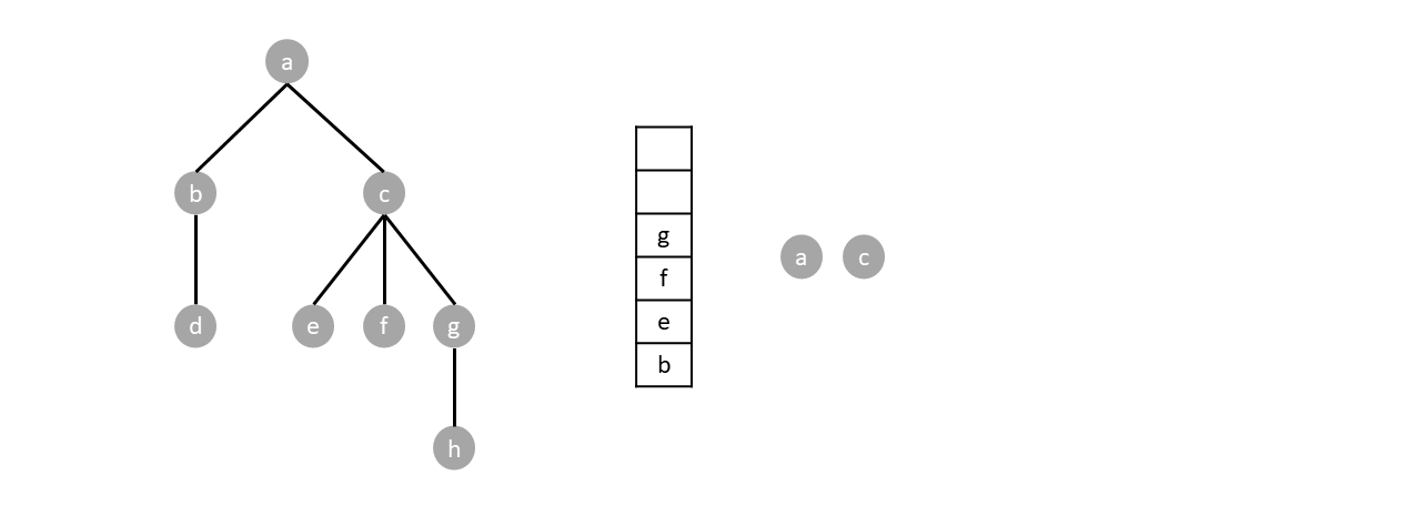
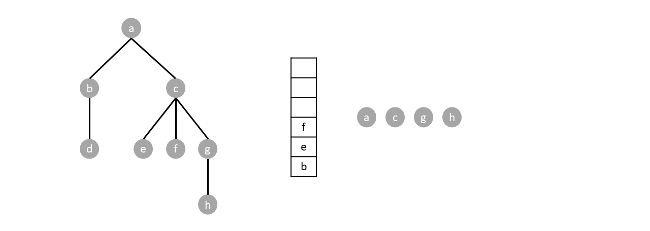
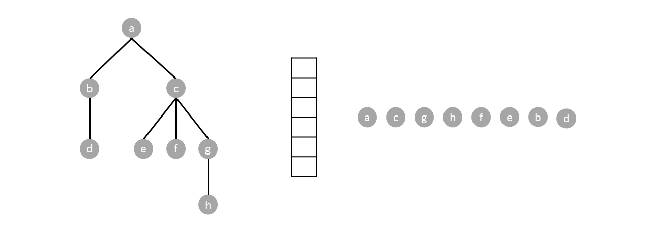
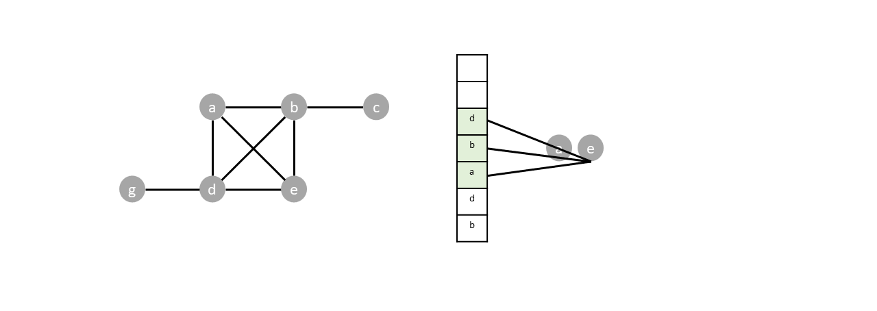
The stack is still not empty so we repeat the process by popping one item (node $c$) and pushing its children.


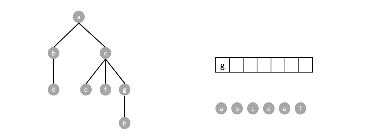
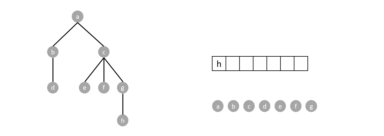
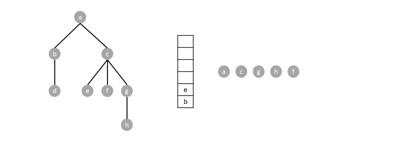
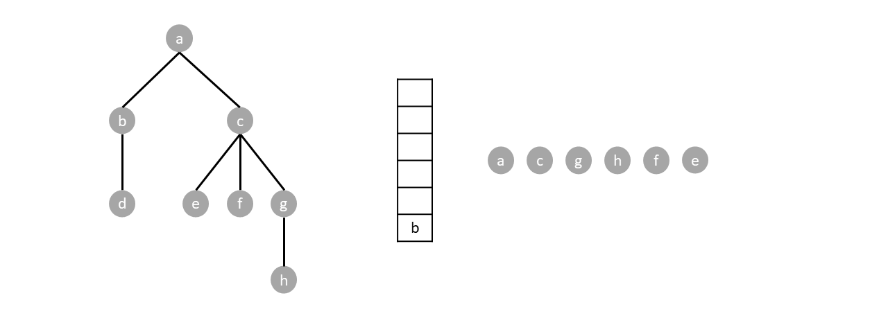
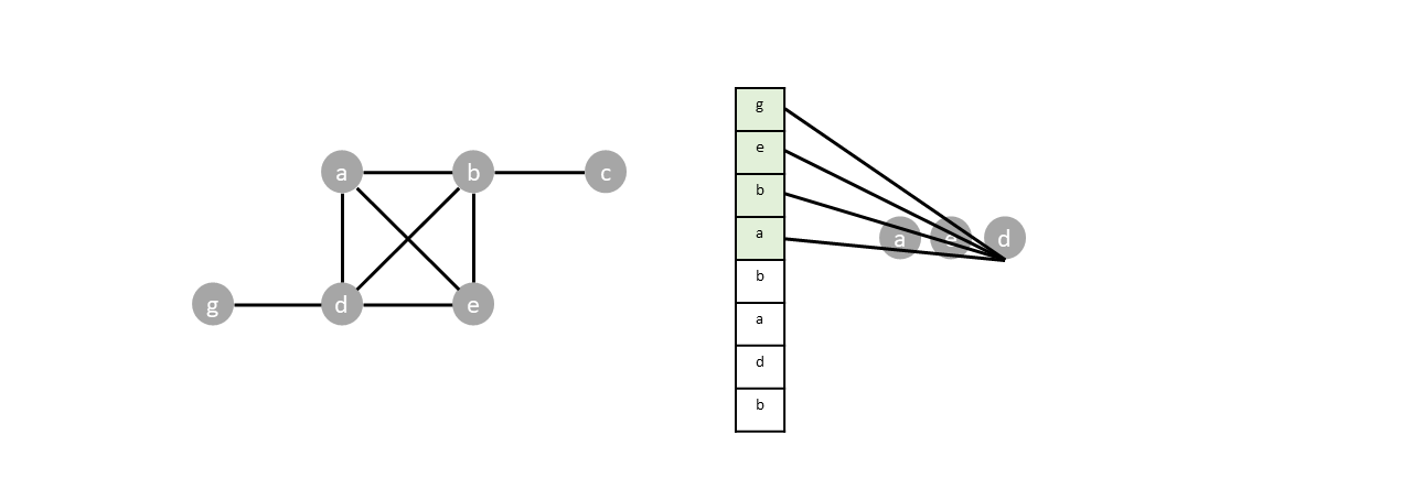
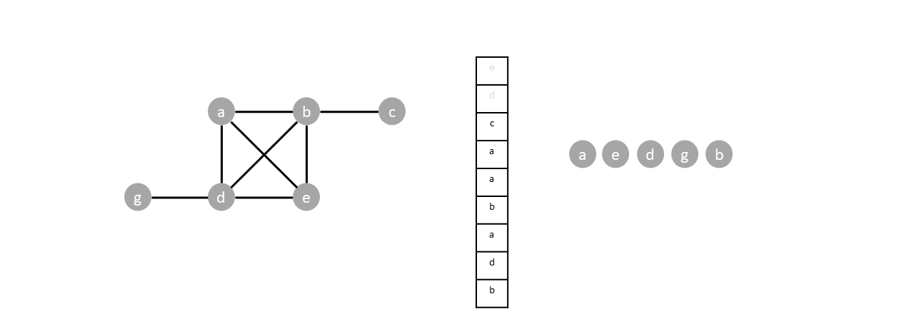
We repeat the algorithm until the stack is empty:







Based when the parent node gets visited, depth first search can either be preorder, postorder or inorder. Preorder traversal visits the parents before any child, postoder visits the parents after all children while inorder visits parents in between the visiting the children.

##### Preorder traversal

The preorder traversal of a rooted tree $T$ is recursively defined as the following,

Visit $T$, then visit each subtree in a preorder manner, from the from the left child to the right child. As a recursive function it works this way:

preorder($T$) = $T$, preorder($T_1$), preorder($T_2$), ..., preorder($T_n$).

> where $T_1,T_2,\cdots ,T_n$ are the subtrees of $T$ ordered from left to right.

For example in the tree below, we start with $a$ then preorder($b$), then preorder($c$).


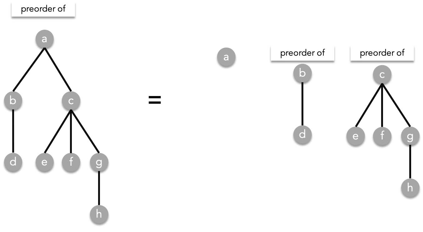
The answer is still not complete since we still need to resolve preorder($b$) and preorder($c$). Since preorder($b$)=($b$, preorder($d$)), resolving that gives us:


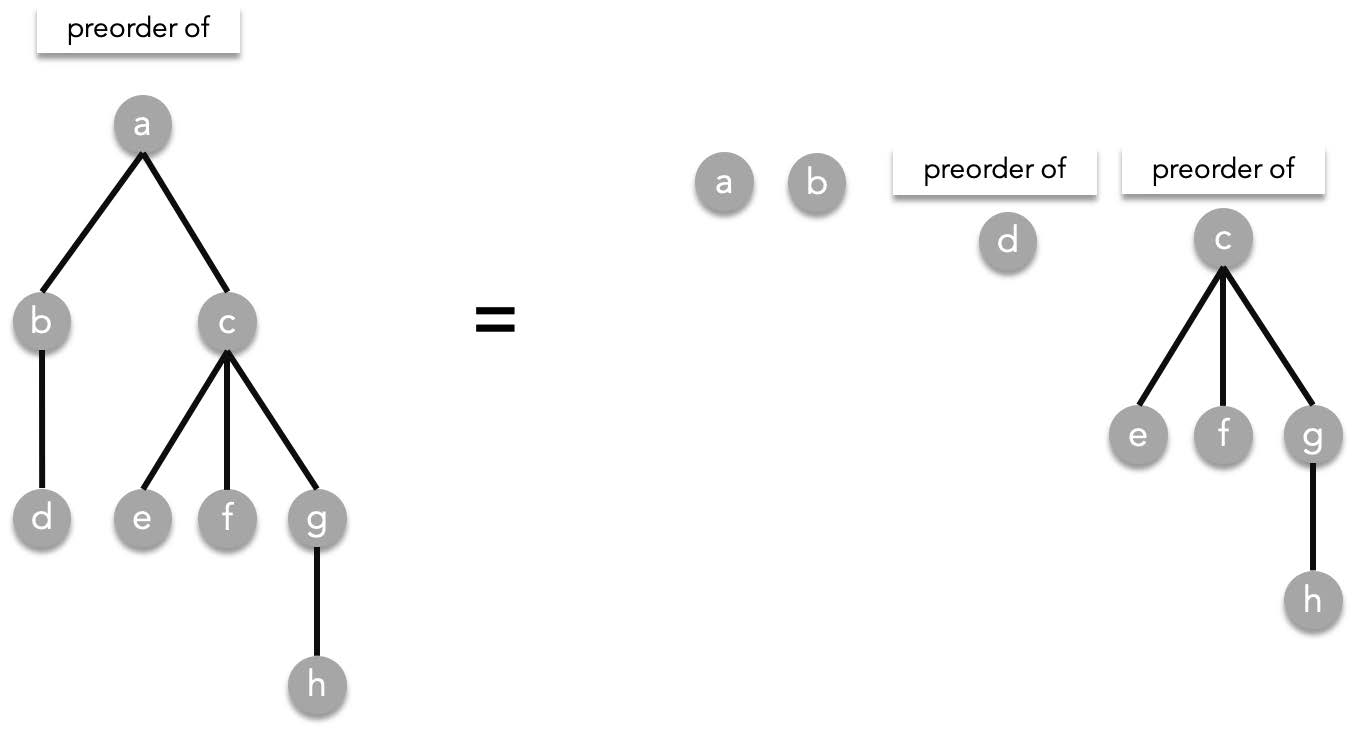
> the order of resolving preorders does not matter, you can try resolving preorder($c$) first and the final result will be the same.

Resolving preorder($d$) is trivial since it does not have children. preorder($d$)=$d$. We resolve that and preorder($c$) as well, which is preorder($c$)=$c$, preorder($e$), preorder($f$), preorder($g$):


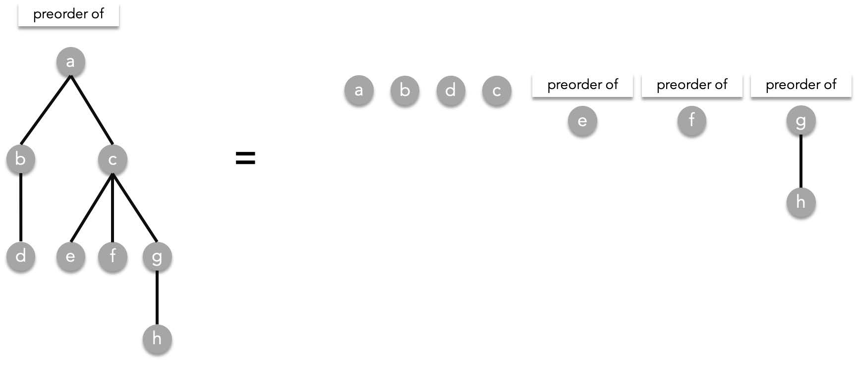
Resolving the following:

- preorder($e$)=$e$
- preorder($f$)=$f$
- preorder($g$)=$g$, preorder($h$)


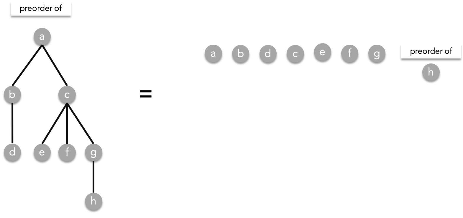
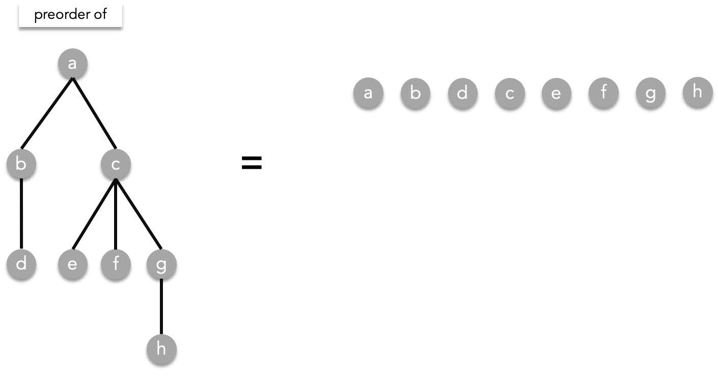
Finally resolving preorder($h$)=$h$:


##### Inorder traversal

Inorder traversal is defined as the following,

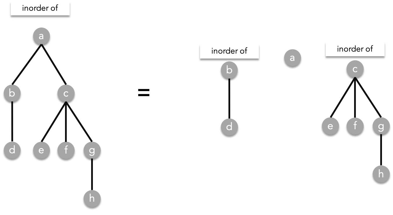
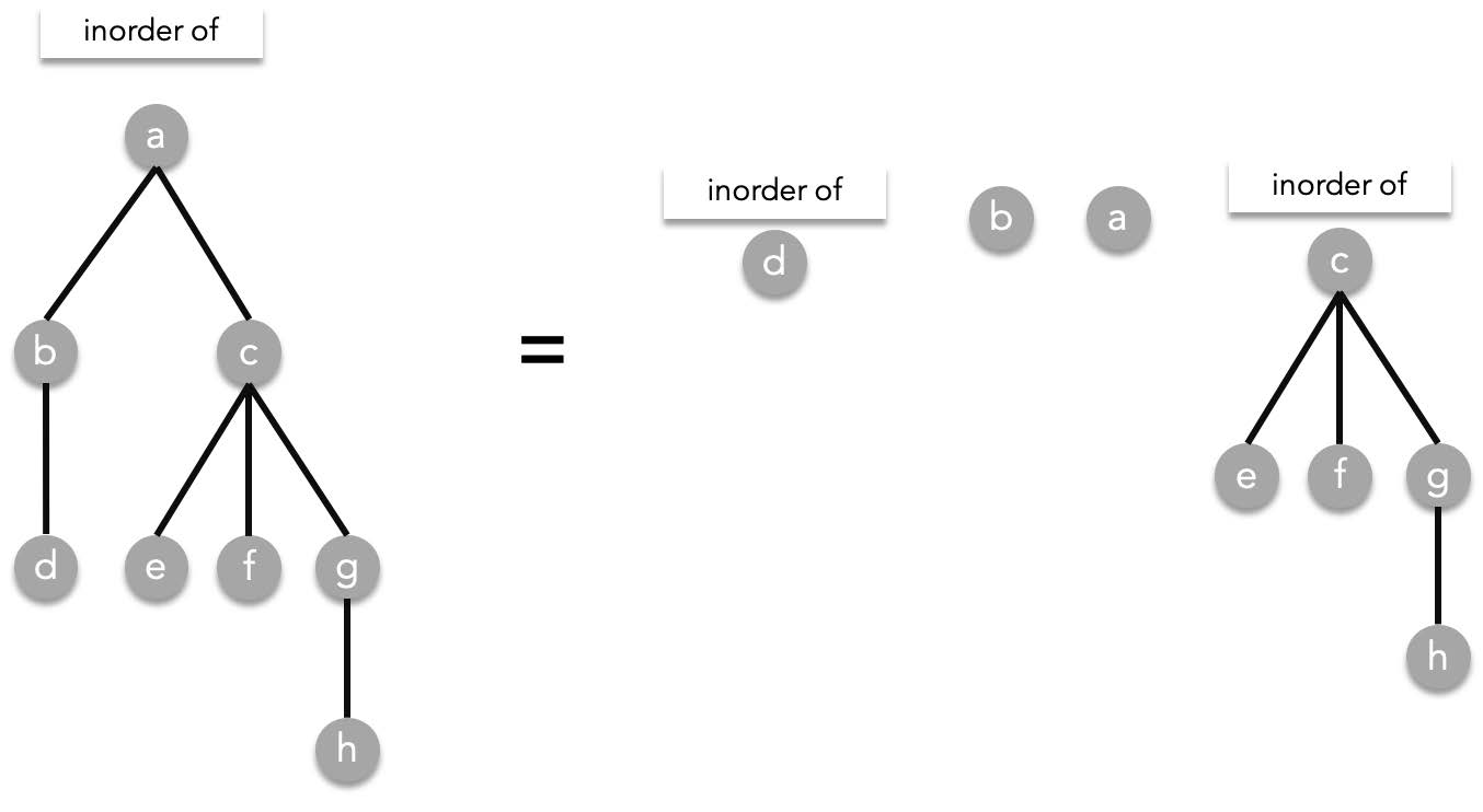
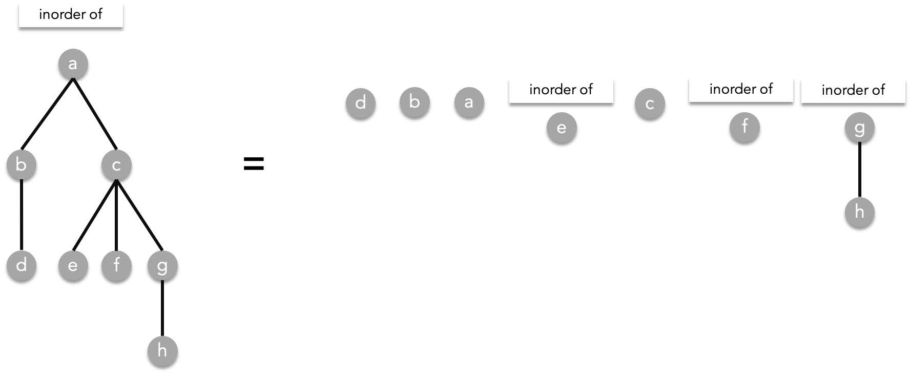
Given the root $T$, visit the leftmost subtree (if it exists) in an inorder manner, visit the root $T$, then visit the other subtrees from left to right. As a recursive function:

Inorder($T$)=Inorder($T_1$), $T$, Inorder($T_2$), Inorder($T_3$), ..., Inorder($T_n$)

> where $T_1,T_2,\cdots ,T_n$ are the subtrees of $T$ ordered from left to right.

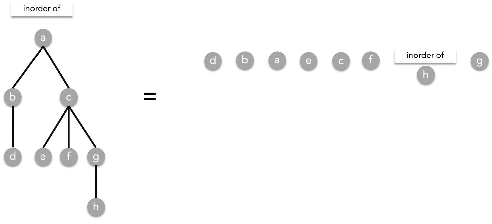
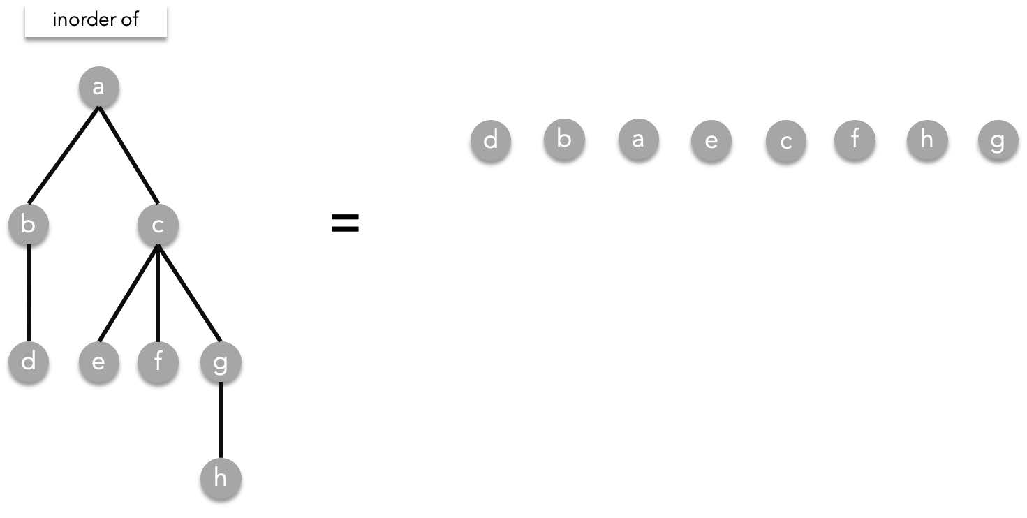
Using the previous tree as an example, inorder works the following way:






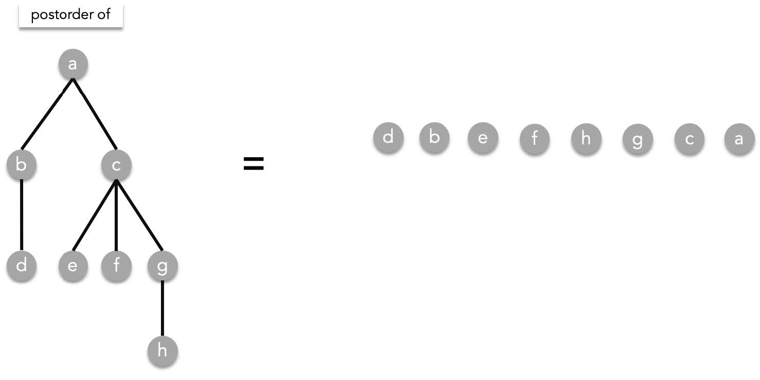
##### Postorder traversal

Postorder is sort of like the opposite of preorder traversal. It is defined as the following.

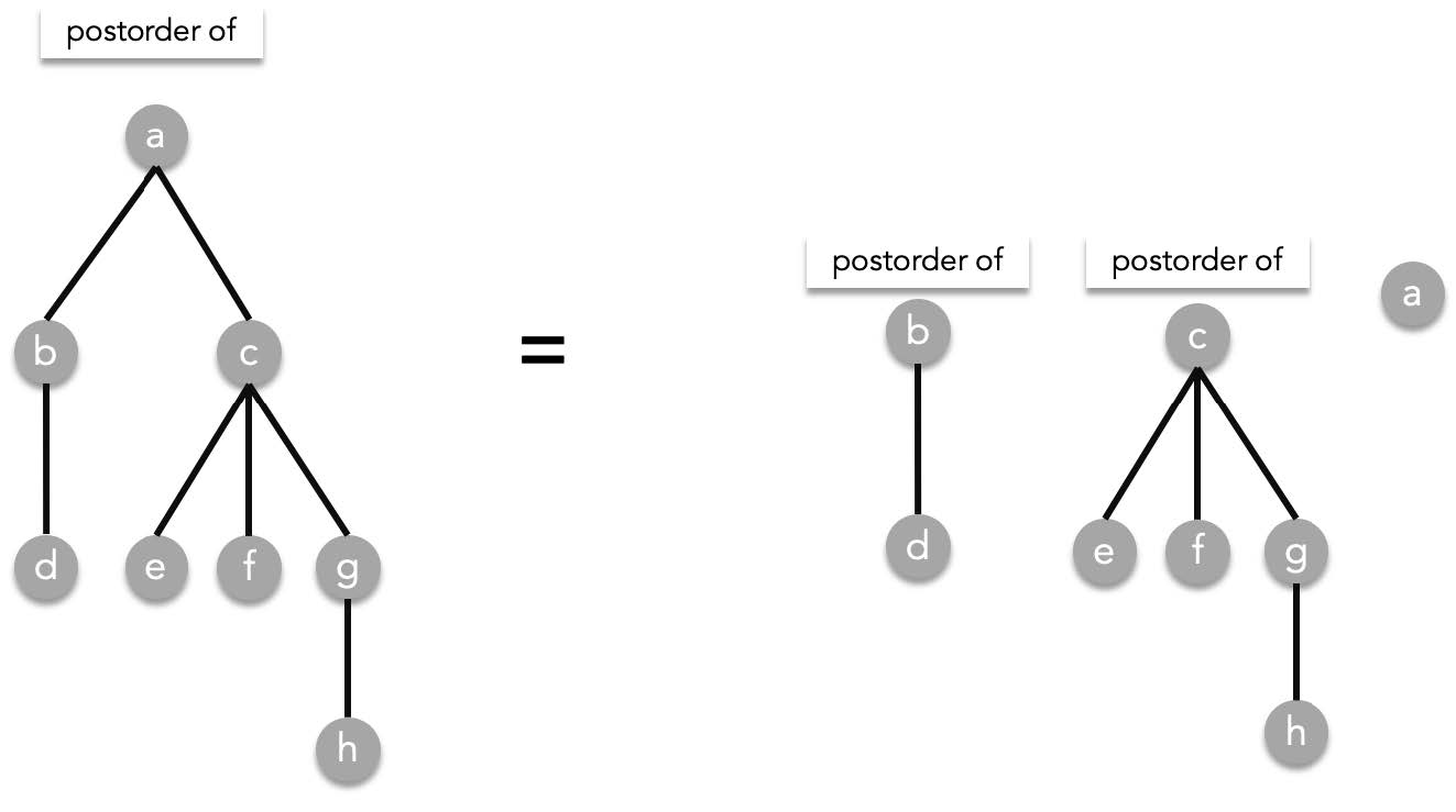
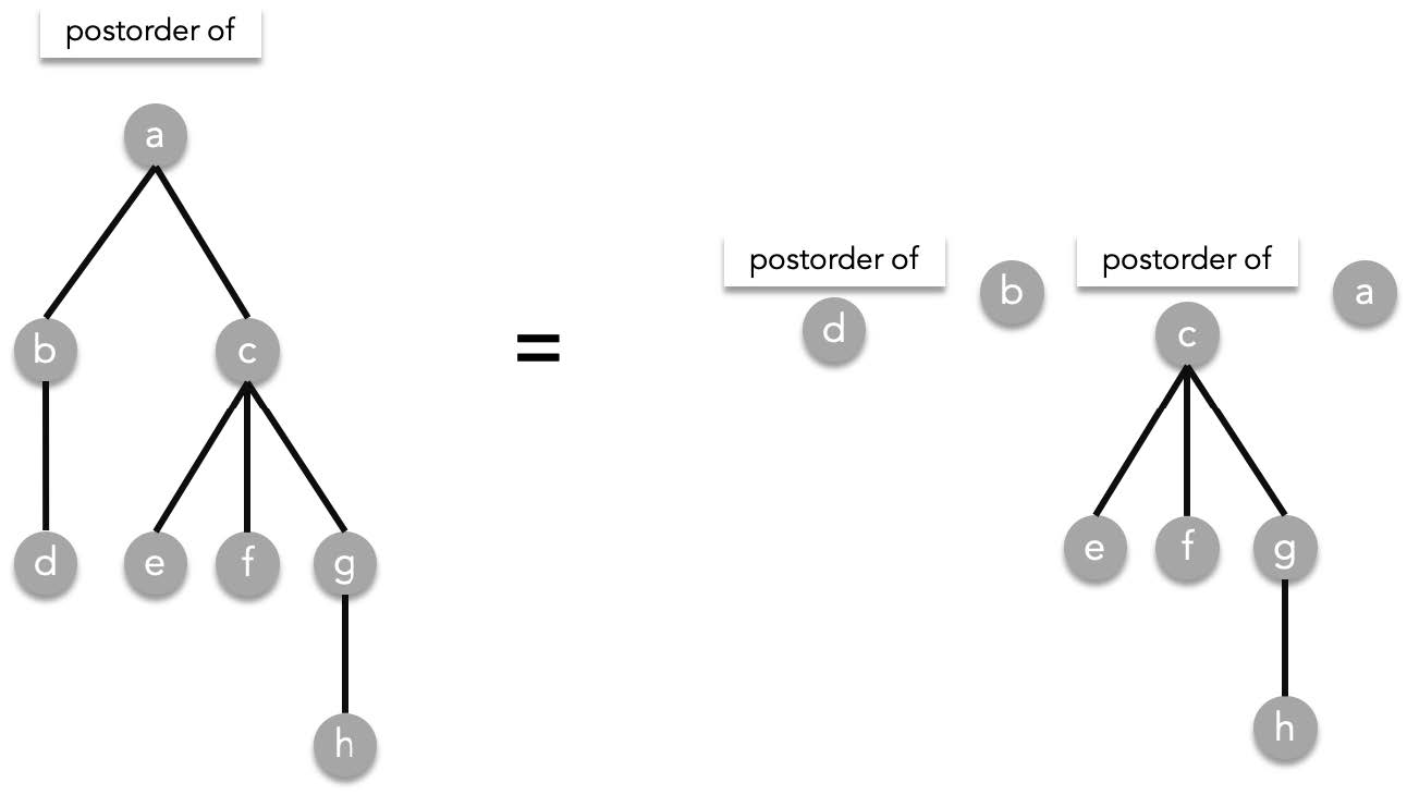
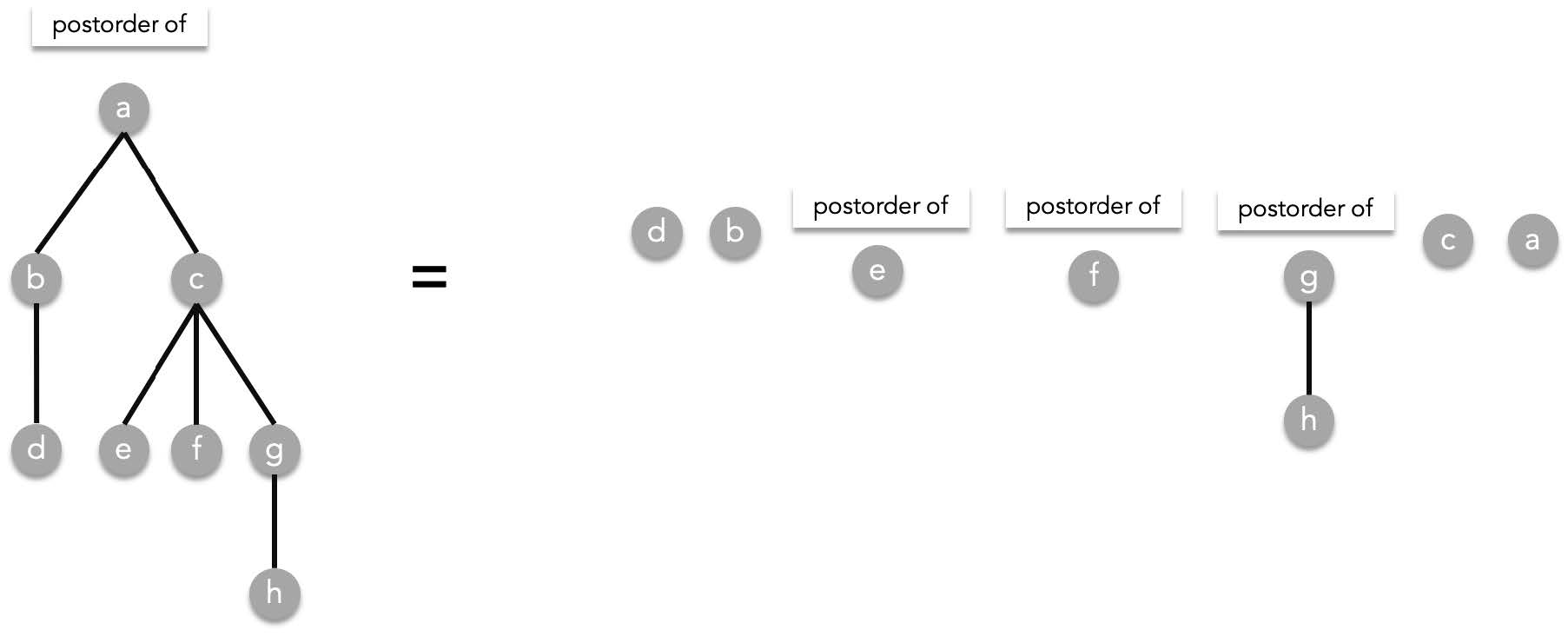
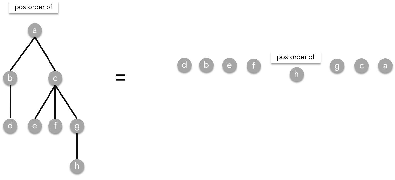
Given a rooted tree $T$, visit all subtrees in a preorder manner from starting from the left to right then visit root T. As a recursive function:

postorder($T$) = postorder($T_1$), postorder($T_2$), ..., postorder($T_n$), $T$.

> where $T_1,T_2,\cdots ,T_n$ are the subtrees of $T$ ordered from left to right.

Using the previous tree as an example:






##### Traversals and expressions

Mathematical expressions can be neatly represented by rooted trees. Consider the expression below,
$$
(2/4)+((3*5)-(4+1))
$$
A mathematical expression such as this is also recursive compositions as well. An expression can be broken down into operands and operators. It is recursive because the operands can either be numbers or expression themselves. Because of this any complicated expression can be represented into a tree. To do this we imagine an operation as a tree. The operands of the operation can either be another expression (a subtree) or a number (a leaf).

Using the expression above we can construct a tree this way. Starting from the sub expression $(2/4)$, we construct the tree:


We also have the expressions $(3*5)$ and $(4+1)$ which are combined via subtraction. Which means we combine $(3*5)$ and $(4+1)$ in a subtraction tree to obtain $((3*5)-(4+1))$


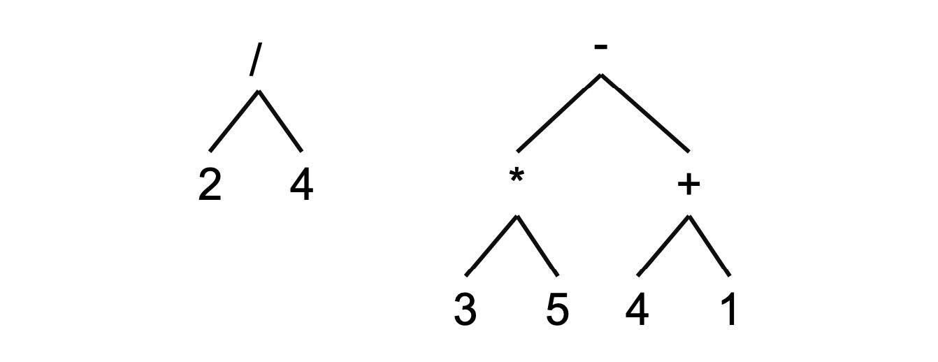
Finally these $(2/4)$ and $((3*5)-(4+1))$ are added together to form $(2/4)+((3*5)-(4+1))$:


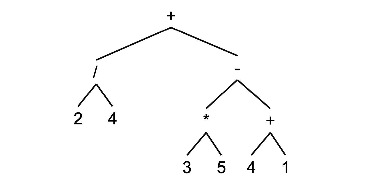
Note that the way we write expressions is actually the inorder traversal of the expression tree. Traversing the tree above will give us:
$$
2/4+3*5-4+1
$$
But because inorder traversal ambiguous, we have to add parentheses to the expression to specify, the exact subtrees of each operator. Thus we end up with $(2/4)+((3*5)-(4+1))$.

> **Ambiguity example**. The following tree is one of the may ways you can interpret the same expression without parentheses:
>
> 

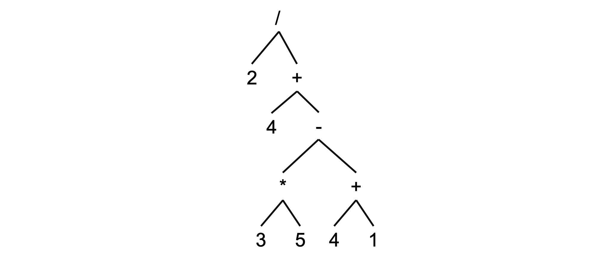
Preorder and postorder traversals however do not have ambiguities. Any preorder/postorder traversals rebuilds into exactly one expression. Therefore, if you write expression using either preorder or postorder, you will not need parentheses. The same expression but preorder and postorder:

- **preorder-** $+,/,2,4, -, *, 3,5, +, 4,1$
- **postorder**- $2,4,/,3,5*,4,1,+,-,+$

> if you try rebuilding these traversals, and you will get the same trees.

### Spanning Trees

Given a connected graph $G=(V,E)$, a spanning tree is a subgraph of $G$ that contains all vertices in $V$ and satisfies the conditions of trees (simple, acyclic and connected).

In the example below, a graph can have multiple spanning trees.


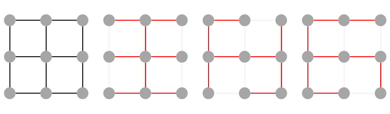
A spanning tree can be found by traversing a connected graph breadth first. You can start from any vertex and avoid forming cycles by making sure each vertex is visited exactly once. Edges are added to the spanning tree whenever children are enqueued.

In the example below, we can form a spanning tree by traversing the graph breadth first using $a$ as the root.


| Queue | Edges added to spanning tree |
| :------ | -----------------------------------------------------------: |
| $a$ | $\{\}$ |
| $b,d$ | $\{\{a,b\},\{a,d\}\}$ |
| $d,c,e$ | $\{\{a,b\},\{a,d\},\{b,c\},\{b,e\}\}$ |
| $c,e,g$ | $\{\{a,b\},\{a,d\},\{b,c\},\{b,e\},\{d,g\}\}$ |
| $e,g,f$ | $\{\{a,b\},\{a,d\},\{b,c\},\{b,e\},\{d,g\},\{c,f\}\}$ |
| $g,f,h$ | $\{\{a,b\},\{a,d\},\{b,c\},\{b,e\},\{d,g\},\{c,f\},\{e,h\}\}$ |
| $f,h$ | $\{\{a,b\},\{a,d\},\{b,c\},\{b,e\},\{d,g\},\{c,f\},\{e,h\}\}$ |
| $h,i$ | $\{\{a,b\},\{a,d\},\{b,c\},\{b,e\},\{d,g\},\{c,f\},\{e,h\},\{f,i\}\}$ |
| $i$ | $\{\{a,b\},\{a,d\},\{b,c\},\{b,e\},\{d,g\},\{c,f\},\{e,h\},\{f,i\}\}$ |
| | $\{\{a,b\},\{a,d\},\{b,c\},\{b,e\},\{d,g\},\{c,f\},\{e,h\},\{f,i\}\}$ |

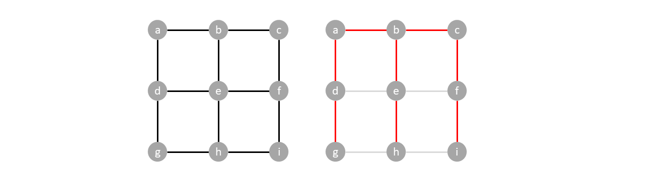
When traversed depth first starting from $a$ it forms a different spanning tree.


Traversing depth first produces a different spanning tree. To avoid cycles in this traversal, you only push children of unvisited edges. Once the order of traversal is found, edges are created by backtracking to closest neighbor.

For example in the graph below we start by designating $a$ as the root, pushing it to the stack:


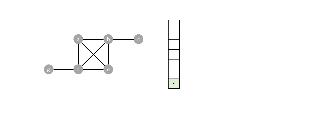
While the stack is not empty we proceed with the algorithm, popping from the stack and pushing the neighbors of each popped vertex.





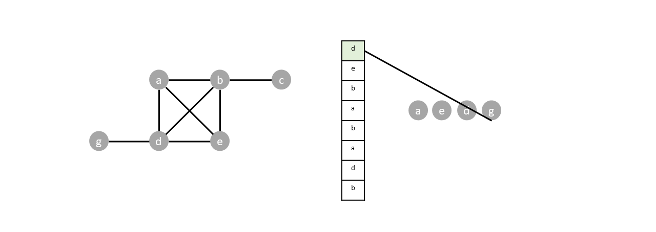
Vertex $d$ and $e$ are popped. But since both vertices are already visited, their neighbors are not pushed into the stack.





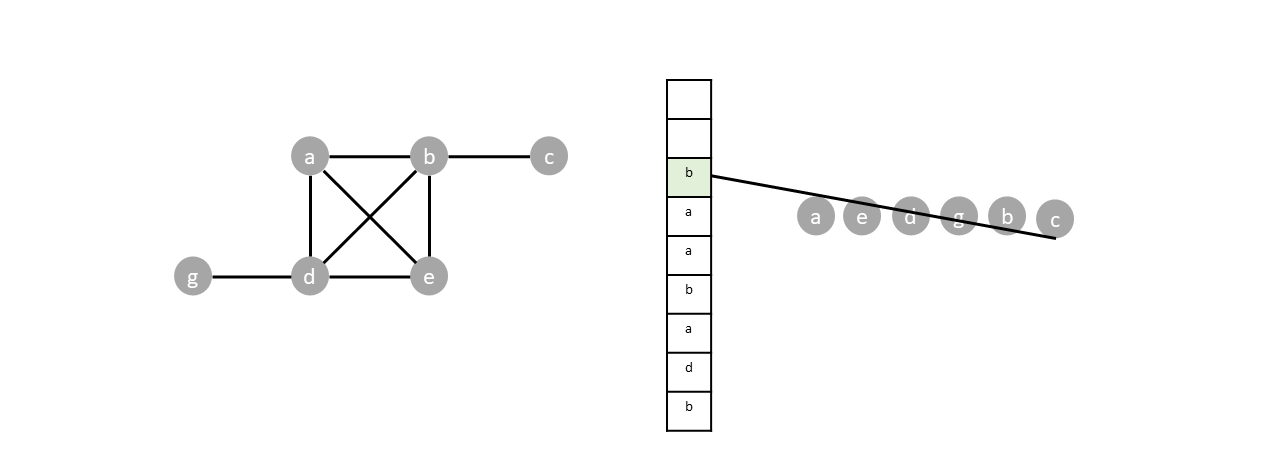
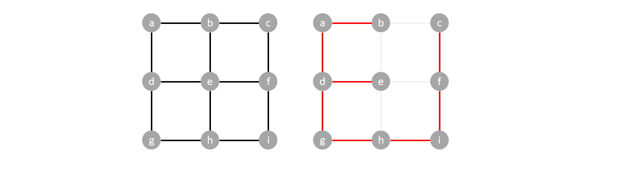
Once the last node is visited ($c$), all items in the stack will be popped without pushing any new vertices, emptying the stack and completing the traversal.


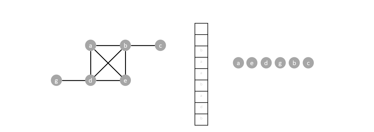
With the traversal sequence known, we build the spanning tree by backtracking from $c$. We connect each vertex to the closest neighboring vertex to the right with respect to the traversal sequence. Vertex $c$ connects to $b$. Vertex $b$ connects to $d$ (since $b$ and $g$ are not neighbors, $b$'s closest neighboring vertex is $d$ in the sequence), and so on until the spanning tree connects to $a$.


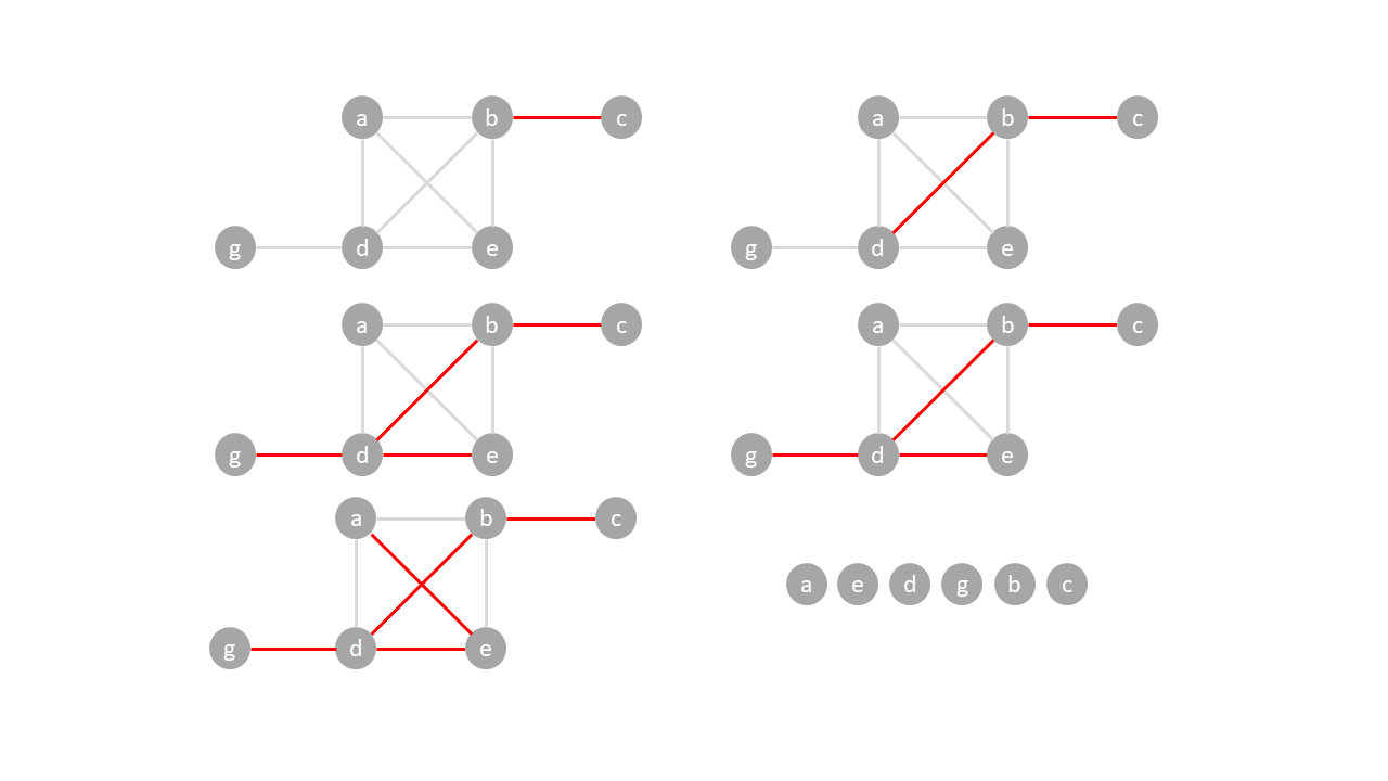
## Minimum spanning tree

Given a weighted graph, the minimum spanning tree is a spanning tree that has the smallest sum of edge weights. In the example below, the top right tree formed from breadth first traversal from $a$ has a total edge weight of $14$. The bottom spanning trees are considered minimum spanning trees, each with a total edge weight of $7$.


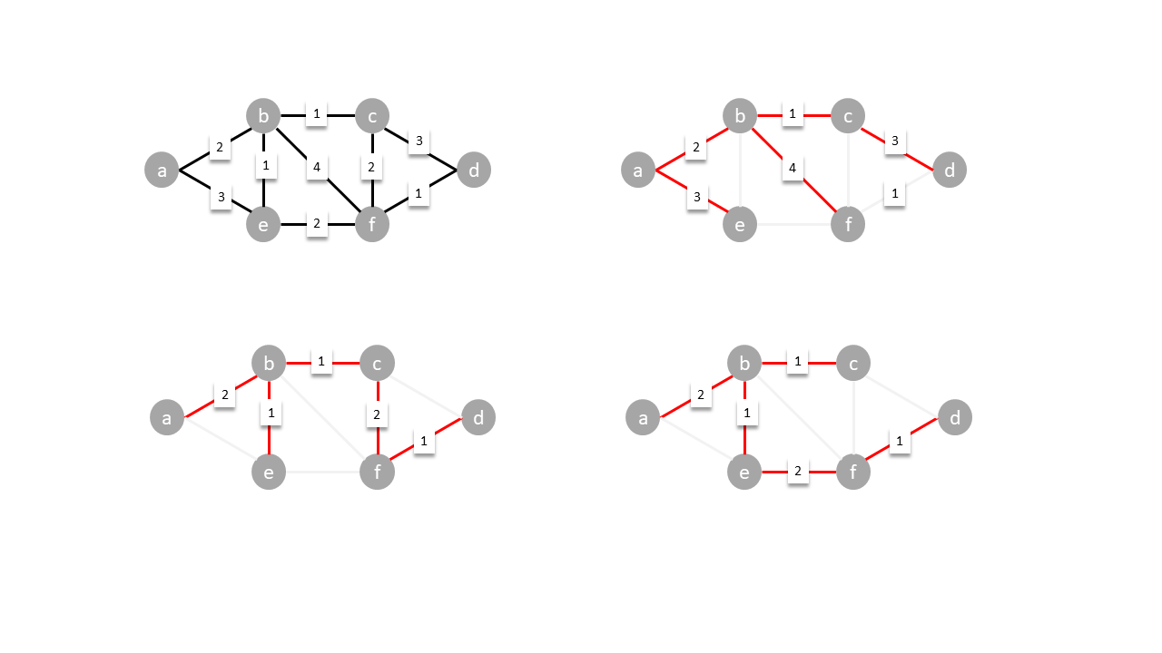
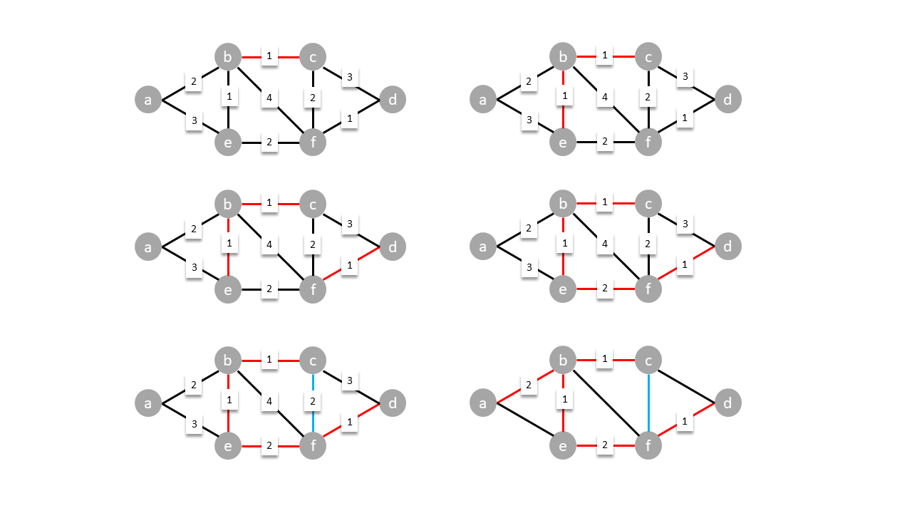
### Kruskal's algorithm

One of the many algorithms used for finding the minimum spanning tree is Kruskal's algorithm. It works by adding the smallest available edge in that doesn't form a cycle until all vertices are connected.

In the diagram below, the smallest edges are added (red), rejecting cycle forming ones (blue), until the all vertices are connected.