---
tags: Communication System Design, ss, ncu
author: N0-Ball
title: Link Equation and Link Budget
GA: UA-208228992-1
---

[ToC]

# Link Equation

:::info
Used to calculate received power in a radio link
:::


Parameters list:
- P~t~ (Transmitted power)
- G (Antenna gains)
- R (Distance between Tx and Rx)
- $f = \frac{c}{\lambda}$ (Radio frequency)

$$
P_r = \frac{\text{EIRP} \times \text{Receiver Antenna Gain}}{\text{Path Loss}}
$$

evaluated in decibels:

$$
P_r = P_t + G_t + G_r - L_p \text{ (dBW)}
$$

Where

P~r~
: Received power in watts

P~t~
: Transmitted power in watts

G~t~
: Transmitting antenna gain (ratio)

G~r~
: Receiving antenna gain (ratio)

L~p~
: Path loss

:::warning
Additional losses must be included in the Link Equation
:::


$$
P_r = P_t + G_t + G_r - L_p - L_a - L_{ta} - L_{ra} \text{ (dBW)}
$$

L~p~
: path loss

L~a~
: loss in atmosphere

L~ta~
: loss in transmitting antenna

L~ra~
: loss in receiving antenna

## Example

: A reciever at **R** and transmitter at source -> the energy consumes

- Isotropic source
- Ideally source that spreads equally
- **R** -> creates area of $4\pi r^2$ sphere **A**
- **ERIP** : source (with unit watt)
- **F** : Flux ($W/m^2$)

:::warning
Temperary not related to frequency
:::

# Receiver

- ***directive*** antentas in satellite systems
- Antenna has a ***narrow*** beam, gain **G** (ratio)
- Gain describes the ability of an antenna to increase power
- **EIRP** (Effective Isotropically Radiated Power) is combination of gain and transmitted power

$$
\text{EIRP} = P_tG_t\ \text{watts}
$$

## Antenna gain

:::info
The increase in received power at a given point with the test antenna relative to the power received from an isotropic antenna, often in dBi (i for isotropic). Ratic of their effective apertures
:::


$$
G = \frac{A_e}{A_{e, i}}
$$

Where $A_e$ is the effective aperture

### Isotropic Antenna

:::info
An antenna that radiates equally in all directions.
:::

Effective aperture of an ideal isotropic antenna is:

$$
A_{e, i} = \frac{\lambda ^2}{4 \pi}
$$

-> Power transferred most efficiently

-> Gain of Isotropic Antenna

$$
G = \frac{4 \pi A_e}{\lambda ^2}
$$

## Received Power


1. for the source **EIRP** = $P_tG_t$ Watt

$$
F = \frac{P_tG_t}{A_s} = \frac{P_tG_t}{4 \pi R^2} \ (W/m^2)
$$

2. Power received, P~r~ by an antenna with an aperture of A m^2^ is

$$
P_r = F \cdot A_e = F \cdot \eta_eA
$$

where $\eta_e$ is related to antenna (effective area)
: often < 1

## Pass Power

$$
\begin{aligned}
P_r &= \frac{P_tG_t}{4 \pi R^2} \cdot \frac{\lambda ^2 G_r}{4 \pi} \\[1em]
&= \frac{\lambda ^2P_tG_tG_r}{(4 \pi R)^2} \ (\text{watt})
\end{aligned}
$$

- Basic Link Equation
- Path Loss
- $L_p = (\frac{4 \pi R}{\lambda})^2$
- How power spreads out with distance
- unavoidable, undeniable, unchangable

## Circular aperture with Diameter D

$$
\begin{aligned}
A &= \frac{\pi D^2}{4} & \because G = \eta_A A \\[1em]
G &= \eta_A (\frac{\pi D}{\lambda})^2 \varpropto (\frac{D}{\lambda})^2
\end{aligned}
$$

## Omni-directional Antennas


- Gain: G < 3dB
- Types:
- dipole
- monopole
- patch
- Patch is printed circuit element, ~ $\frac{\lambda}{2}$

* Left is Dipole and right is Monopole

## Low Gain Antennas

- Gain: 3dB < G < 25dB
- Used as reflector antennas and sometimes elements in phased arrays
- Types
- horn
- Yagi-Uda
- helical

## High Gain Antennas

- Gain: 30dB < G < 100dB
- Reflectors, phased arrays, lenses (rare)
- Aperture antennas
- Create uniform phase distribution over aperture -> how we get G
- Far-field pattern has main lobe and side lobes


## Antenna Pattern

Pattern
: directional dependence of the strength of the radio waves form the source


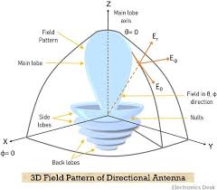
* Can be three-directional or two-directional

Beamwidth
: measured between -3 dB (half of power) points of antenna pattern

$$
\theta = \frac{51 ^ \circ \lambda}{D} \sim \frac{ 75 ^ \circ \lambda}{D} \varpropto \frac{\lambda}{D}
$$

# Gain and Directivity

Directivity
: Maximum power density $P(\theta, \phi)_{max}$ to its average value over a sphere as observed in the far field of an antenna

$$
D = \frac{4 \pi}{\Omega_A}
$$

* A_e is 60% ~ 65%

:::info
Apporoximate formula for G(empirical)
:::
$$
G = \frac{33000}{\theta_a \theta_b}
$$

where $\theta_a$ and $\theta_b$ are antenna beamwidths in degrees in two orthogonal panes

# Propagation

- free space follows path loss law
- is proportional to **square of distance** from transmitter
- Additional losses occur if link is not on line of sight (LOS)
- Mobile radio (cellphones) and indoor wireless systems (Wi-Fim WLans) suffer *multipath* and blockage

$\Rightarrow$ Leads to comples propagation models

:::warning
- Most links at microwave frequencies (> 1GHz rely on LOS propagation)
- Cellular phone designers use R^4^ law (path loss $\varpropto$ R^4^) with statistical variation to account for multipath
- Atmospheric losses occur at microwave frequencies
- Rain is most important factor above 10 GHz
:::

## In Earth's Atmosphere

- Designed to withstand a specific attenuation
- Maximum permitted attenuation is called **link margin**
- attenuation excceds link margin -> suffers an outage(inaccessible)
- Percentage time for which signal is above minimal link margin is called **link availability**

# Link budgets
- usually tabulated in dB
- tabulated in a similar way as a financial budget
- parameters left
- value right
- Bottom line
- P~r~ for received power budget
- P~n~ for noise power budget

:::danger
Keep **received power** and **noise power** budgets separate
:::

- Then calculate C/N = P~t~/P~n~ in dB

## Example

:::info
Geo Satellite:
- Altitude = 40,000km
- Downlink at wavelength $\lambda = 0.075 (m), 4GHz$
Satellite:
- P~t~ = 20W or 13 dBW
- G~t~ = 20dB
Earth Station:
- G~r~ = 40dB
Path:
- Atmospheric loss in clear air = 0.3dB
- Miscellaneous losses = 0.5dB
:::

$$
\begin{aligned}
L_p = (\frac{4 \pi R}{\lambda})^2 = (\frac{4 \pi \cdot 4 \times 10 ^ 7}{7.5 \times 10 ^ {-2}})^2 \sim 4.5 \times 10 ^ {19} (W) = 10 \times log_{10}(4.5 \times 10 ^{19}) dBW \sim 196.5 dBW
\end{aligned}
$$

| Parameter | Value |
| --------- | ------- |
| P~t~ | 13dB |
| G~t~ | 20dB |
| G~r~ | 40dB |
| L~p~ | -196.5dB |
| L~a~ | -0.3dB |
| L~m~ | -0.5dB |
| Sum | -124.3dB |

# Summary

## No Loss

$$
P_r = P_t + G_t + G_r - L_p \text{ (dBW)}
$$

## With Loss

$$
P_r = P_t + G_t + G_r - L_p - L_a - L_{ta} - L_{ra} \text{ (dBW)}
$$

## EIRP
:::warning
with no lost
:::

### Watts
$$
EIRP = P_t \times G_t \\[1em]
P_r = \frac{EIRP \times G_r}{L_p}
$$

### dBW
$$
EIRP = P_t + G_t \\[1em]
P_r = EIRP + G_r - L_p
$$

## Antennas


# Extra

## Effective Aperture (TBD)