# Model Cheking 3
去年の資料
https://ryutaro-kodama.github.io/slides/semi/journal_club/ModelChecking_ch3/
## 目的
* システム(プログラム)の正しさを検証するために
* 正しさ=システムが持つべき特徴(specification)の定式化
* システム(プログラム)のmodel化
3章はmodel化について
----
## モデルを作る際のポイント
* 適切に抽象化する
* **特徴(specification)に影響を与える部分の**モデルは正確である(現実のシステムをよく表している)べき
* 与えない部分は抽象化する
* 例 デジタル回路のmodel化: 電圧ではなく、その解釈のbool値を考える
* 例 communication protocolのmodel化: 暗号化やネットワーク上でのバイナリ列は考えず、protocol階層でのメッセージを考える。
* 「無かったことにする」のではなく、summary(入力と出力の関係)を考える
* 内部状態を考える
* プログラムを想定すると、入力には多くのパターンがある
* そのため、単にinput-outputに応じたモデルを構築するのは困難
* $\{f(00)=1,f(10)=2,f(30)=3,\dots\}$
* 状態(state)と、状態遷移(transition)を考えることで解決
----
## Transition System
### Transition System
transition system $T = (S,S_0, R)$
* $S$: 状態の集合(断りが無い限りは有限集合)
* $S_0$: 初期状態の集合 ($S_0 \subseteq S$)
* $R$: 状態遷移 ($R \subseteq S\times S$, left total)
* $s$から$s'$に遷移するとき、$(s,s') \in R$であり、$R(s,s')$とかく。
* left total: 全ての$s$についてその遷移先がある $\forall s \in S, \exists s' \in S, R(s,s')$
----
### 例1
* $S = \{s_0,s_1,s_2\}$:
* $S_0 = \{s_0\}$:
* $R = \{(s_0,s_1), (s_1,s_0), (s_2,s_1)\}$
```graphviz
digraph def_graph {
// the first layer
start [shape = none, label = ""];
S0 [label = "S0"];
S1 [label = "S1"];
S2 [label = "S2"];
start -> S0
S0 -> {S1}
S1 -> {S0}
S2 -> {S1}
}
```
----
### 例2
* $S = \{s_0,s_1,s_2\}$:
* $S_0 = \{s_0\}$:
* $R = \{(s_0,s_1), (s_1,s_2), (s_2,s_1)\}$
Q. 遷移はどうなる?
```graphviz
digraph def_graph {
// the first layer
S0 [label = "S0"];
S1 [label = "S1"];
S2 [label = "S2"];
}
```
<details>
<summary>答え</summary>
```graphviz
digraph def_graph {
// the first layer
start [shape = none, label = ""];
S0 [label = "S0"];
S1 [label = "S1"];
S2 [label = "S2"];
start -> S0
S0 -> {S1}
S1 -> {S2}
S2 -> {S1}
}
```
</details>
----
### path
finite path(有限パス)
* $p=s_0,s_1,\dots,s_n$ ($R(s_i,s_{i+1})$)
infinite path(無限パス)
* $p=s_0,s_1,\dots$ ($R(s_i,s_{i+1})$)
----
## Kripke structure
各状態にlabelをつけたTransition System
### Kripke structure
Kripke structure $M = (S,S_0, R, AP, L)$
* $S,S_0,R$はTransition Systemと同じ
* $S$: 状態の集合(断りが無い限りは有限集合)
* $S_0$: 初期状態の集合 ($S_0 \subseteq S$)
* $R$: 状態遷移 ($R \subseteq S\times S$, left total)
* $AP$: atomic propositionの全体集合
* $L$: ある状態でtrueなatomic propositionの集合を得る関数 ($S \to 2^{AP}$)
### atomic proposition と state label
stateの持つ性質の一つ一つを、atomic proposition(原子命題)、又は、labelという。
> We refer to these labels as atomic propositions
例:
* p: 変数aが0に等しい
* q: 変数bが1に等しい
$L$の例:
$L = \{s_0 \mapsto \{p\}, s_1 \mapsto \{p,q\}\}$
----
### 例1
* $S = \{s_0,s_1,s_2\}$:
* $S_0 = \{s_0\}$:
* $R = \{(s_0,s_1), (s_1,s_0), (s_2,s_1)\}$
* $AP = \{p,q\}$
* $L = \{s_0 \mapsto \{p\}, s_1 \mapsto \{p,q\}, s_2 \mapsto \emptyset\}$
```graphviz
digraph def_graph {
// the first layer
start [shape = none, label = ""];
S0 [label = "S0\np"];
S1 [label = "S1\np,q"];
S2 [label = "S2\n∅"];
start -> S0
S0 -> {S1}
S1 -> {S0}
S2 -> {S1}
}
```
----
### 例2
* $S = \{s_0,s_1,s_2\}$:
* $S_0 = \{s_0\}$:
* $R = \{(s_0,s_1), (s_1,s_2), (s_2,s_1)\}$
* $AP = \{p,q\}$
* $L = \{s_0 \mapsto \{p\}, s_1 \mapsto \emptyset, s_2 \mapsto \{p,q\}\}$
Q. labelはどうな
```graphviz
digraph def_graph {
// the first layer
start [shape = none, label = ""];
S0 [label = "S0"];
S1 [label = "S1"];
S2 [label = "S2"];
start -> S0
S0 -> {S1}
S1 -> {S0}
S2 -> {S1}
}
```
<details>
<summary>答え</summary>
```graphviz
digraph def_graph {
// the first layer
start [shape = none, label = ""];
S0 [label = "S0\np"];
S1 [label = "S1\n∅"];
S2 [label = "S2\np,q"];
start -> S0
S0 -> {S1}
S1 -> {S0}
S2 -> {S1}
}
```
</details>
----
### ※補足
文脈によってkripke structureが表すmodelが異なる
* model checkingの文脈: 解析対象のシステムのmodel
* 論理学の文脈: 仕様のmodel
---
## Nondeterminism (非決定性)
ある状態に対し、2つ以上の遷移可能な次状態が存在すること。
初期状態が2つ以上ある場合を含む。
外界からの入力を扱ったり、乱数をあつかったりする場合におこる。
----
### 例: 電気のスイッチ
* 0: 電気が消えている
* 1: 電気がついている
* p: ボタンが押されている
* r: ボタンが押されていない
* 非決定性
* 初期状態: ボタンを押しているか・押していないかは分からない
* 状態遷移: ボタンをそのままにするか・しないかはわからない

<!--
```graphviz
digraph def_graph {
// the first layer
start0 [shape = none, label = ""];
start1 [shape = none, label = ""];
S0 [label = "0,p"];
S1 [label = "0,r"];
S2 [label = "1,r"];
S3 [label = "1,p"];
start0 -> S0
start1 -> S1
S0 -> {S0,S1}
S1 -> {S1,S2}
S2 -> {S2,S3}
S3 -> {S0,S3}
}
```
-->
---
## state の表現
### informal 一階述語論理(first-order logic)
個体の量化のみを許す(述語論理上の関数の量化はない)述語論理。
プログラムを考えると、変数が量化できるので殆どの state を表現することができる。
今回使うのは$\wedge,\vee,\neg,\implies,\forall,\exists$
今後の状態遷移を考える上で、 state が一階述語論理で表現されているとすると嬉しい。
(本質的な問題ではない)
### first-order logic で state 集合を表現
元々の state (valuation): $V \to D$
$V$: 変数集合
$D$: 変数の定義域
変数とその値のマッピング。
ある一階述語論理の式には、その式が true となる全ての state 集合が対応する。
state 集合 $A$ について、$A$に対応する式が$\varphi$であるとき、
$(s \in A) \iff (s \models \varphi)$
#### 例1
$V = \{v_1, v_2, v_3\}$
元々の state (valuation) 集合の書き方
$$
\begin{aligned}
\{<v_1 \mapsto 1, v_2 \mapsto 2, v_3 \mapsto 5>\}
\end{aligned}
$$
first-order logic を使った state の書き方
$$
\begin{aligned}
(v_1 = 1) \wedge (v_2 = 2) \wedge (v_3 = 5)
\end{aligned}
$$
#### 例2
$V = \{v_1, v_2, v_3\}$
元々の state の書き方
$$
\begin{aligned}
\{&<v_1 \mapsto 1, v_2 \mapsto 2, v_3 \mapsto 5>,\\
&<v_1 \mapsto 1, v_2 \mapsto 2, v_3 \mapsto 6>,\\
&<v_1 \mapsto 1, v_2 \mapsto 2, v_3 \mapsto 7>\}
\end{aligned}
$$
first-order logicを使ったstateの書き方
$$
\begin{aligned}
(&((v_1 = 1) \wedge (v_2 = 2) \wedge (v_3 = 5)) \vee\\
&((v_1 = 1) \wedge (v_2 = 2) \wedge (v_3 = 6)) \vee\\
&((v_1 = 1) \wedge (v_2 = 2) \wedge (v_3 = 7)) )
\end{aligned}
$$
### first-order formula を使うメリット1: 式の単純化
一階述語論理のまま、式を単純にできることがある。
$$
\begin{aligned}
&((v_1 = 1) \wedge (v_2 = 2) \wedge (v_3 \geq 5) \wedge (v_3 \leq 7))
\end{aligned}
$$
### first-order formula を使うメリット2: 集合演算が一階述語論理に閉じている
* $A,B$: 状態集合
* $\varphi_A,\varphi_B$: 対応する一階述語論理
* $(s \in A) \iff (s \models \varphi_A)$
* $(s \in B) \iff (s \models \varphi_B)$
|集合演算|論理式演算|補足|
|-|-|-|
|$A \cup B$|$\varphi_A \vee\varphi_B$|$(s \in A\cup B) \iff (s \models \varphi_A\vee\varphi_B)$|
|$A \cap B$|$\varphi_A \wedge\varphi_B$|$(s \in A\cap B) \iff (s \models \varphi_A\wedge\varphi_B)$|
|$S \setminus A$|$\neg\varphi_A$|$(s \in S \setminus A) \iff (s \models \neg\varphi_A)$|
|$A \subseteq B$|$\varphi_A \implies \varphi_B$|$(A \subseteq B) \\\iff (\forall s\in S, s \in A \implies s \in B) \\\iff (\forall s\in S, s \models \varphi_A \implies s \models \varphi_B)$|
---
## transition の表現
### first-order logic で transition を表現
遷移前の変数と、遷移後の変数を区別する必要がある。
遷移後の変数集合を$V'$と書く。各変数についても同様。
* $V = \{v_1,v_2\}$であれば、$V' = \{v'_1,v'_2\}$
以下のように transition の 論理式表現$\mathcal{R}$を定義
$$
R(s,s') \iff (s,s' \models \mathcal{R}) \iff ((\varphi_{\{s\}} \wedge \varphi'_{\{s'\}}) \implies \mathcal{R})
$$
### イメージ例
$\mathcal{R} := (v'_1 = v_1) \wedge (v'_2 = v_2 + 1)$
のとき、例えば
$s \in (v_1 = 1 \wedge v_2 = 1 \wedge v_3 = 0), s' \in (v'_1 = 1 \wedge v'_2 = 2)$は$R(s,s')$
※この$\mathcal{R}$だと、状態数有限かつleft totalにならない。実際はもっと複雑な式が必要。
---
## Kripke 構造の一階述語論理表現
Kripke 構造 $M = (S,\mathcal{S}_0, \mathcal{R}, AP, L)$
* $S$: stateの集合
* すなわち、Vの各変数とその値のマッピング、の集合
* $\mathcal{S}_0$: 初期状態の集合を表す論理式
* $S_0$: 初期状態の集合 $S_0 \subseteq S$について、$\forall s, (s_0 \in S_0) \iff (s_0 \models \mathcal{S}_0)$
* $\mathcal{R}$: 状態遷移を表す論理式
* $R$: 状態遷移 ($R \subseteq S\times S$, left total)について、$R(s,s') \iff (s,s' \models \mathcal{R})$
* $AP$: atomic propositionの全体集合
* $L$: ある状態でtrueなatomic propositionの集合を得る関数 ($S \to 2^{AP}$)
### 例
* $D$(変数の定義域)$= \{0,1\}$
* $V=\{x,y\}$
* $S = \{(0,0),(0,1),(1,0),(1,1)\}$※(x,y)の形式でstateを表現
* $\mathcal{S}_0 = (x=1 \wedge y=1)$
* $\mathcal{R}((x,y),(x',y')) = (x' = (x+y)\text{mod} 2 \wedge y'=y)$
```graphviz
digraph def_graph {
// the first layer
start0 [shape = none, label = ""];
S0 [label = "0,0"];
S1 [label = "0,1"];
S2 [label = "1,0"];
S3 [label = "1,1"];
start0 -> S1
S0 -> {S0}
S1 -> {S3}
S2 -> {S2}
S3 -> {S1}
}
```
### Boolean Encoding
$D$(変数の定義域)$= \{0,1\}$のとき、$v$を論理式上のbool変数とすることで
* $v=0$を$\neg v$
* $v=1$を$v$
と略記したような結果が得られる。
* $D$(変数の定義域)$= \{0,1\}$
* $V=\{x,y\}$
* $S = \{(0,0),(0,1),(1,0),(1,1)\}$※(x,y)の形式でstateを表現
* $\mathcal{S}_0 = (x=0 \wedge y=0)$
$$
\begin{aligned}
\mathcal{R}((x,y),(x',y')) &= (\neg x \wedge \neg y \wedge x' \wedge \neg y')\\
&\vee (x \wedge \neg y \wedge y')&\text{※辺を二本纏めて表現}\\
&\vee (\neg x \wedge y \wedge \neg x' \wedge \neg y')\\
&\vee (x \wedge y \wedge x' \wedge y')\\
\end{aligned}
$$
```graphviz
digraph def_graph {
// the first layer
start0 [shape = none, label = ""];
S0 [label = "0,0"];
S1 [label = "1,0"];
S2 [label = "0,1"];
S3 [label = "1,1"];
start0 -> S0
S0 -> {S1}
S1 -> {S2,S3}
S2 -> {S0}
S3 -> {S3}
}
```
## 例: Modeling Digital Circuits
論理回路のモデリング
### Synchronous circuits
同期回路
register が0/1の値を持っている。
クロックに従い、各レジスタが同時に更新される。
#### 例 mod8 カウンタ
$V = \{v_0,v_1,v_2\}$

$\mathcal{R}$を算出してみる。
それぞれの変数の変化に注目すると、
$$
\begin{aligned}
\mathcal{R}_0 &:= (v'_0 \iff \neg v_0)\\
\mathcal{R}_1 &:= (v'_1 \iff v_0 \text{ xor } v_1)\\
\mathcal{R}_2 &:= (v'_2 \iff (v_0 \wedge v_1) \text{ xor } v_2)\\
\end{aligned}
$$
これらを纏めた結果が$\mathcal{R}$になる。
$\mathcal{R} = \mathcal{R}_0 \wedge \mathcal{R}_1 \wedge\mathcal{R}_2 \\\quad= (v'_0 \iff \neg v_0) \wedge(v'_1 \iff v_0 \text{ xor } v_1)\wedge(v'_2 \iff (v_0 \wedge v_1) \text{ xor } v_2)$
#### $\mathcal{R}$ の一般的な構築
n レジスタのデジタル回路のモデル化
各変数について、その変化を表す関数が回路から作れる。
$$
\mathcal{R}_i := \begin{cases}
true \quad\text{ 値が入力によって決まる場合}\\
(v'_i \iff f_i(V)) \quad\text{otherwize}
\end{cases}
$$
これらの$\wedge$をとれば遷移が得られる
$$
\mathcal{R} := \bigwedge_i \mathcal{R}_i
$$
### Asynchronous Circuits
非同期回路
wire が0/1の値を持っている。
各導線上を流れる電流が、非同期に更新される。
同期回路では同時に更新が行われたが、非同期回路では同時ではない更新=一つだけが更新されることが繰り返される、と捉えることが出来る。
$$
\mathcal{R} := \bigwedge_i \mathcal{R}_i\\
\mathcal{R}_i := \begin{cases}
true \quad\text{ 値が入力によって決まる場合}\\
(v'_i \iff f_i(V))\wedge\bigwedge_{j\neq i} (v'_j\iff v_j) \quad\text{otherwize}
\end{cases}
$$
$\bigwedge_{j\neq i} (v'_j\iff v_j)$で、他の変数が同時に更新されない(interleaving semantics)を表現している。
非同期回路に限って言えばinterleaving semanticsでなくても良いはずだが、今後の議論を簡単にするため?
### 例題
$V = \{v_0,v_1\}$
$v_0' = v_0\text{ xor }v_1, v_1' = v_0\text{ xor }v_1$
$S_0 = (v_0 \wedge v_1)$
同期の場合の遷移
```graphviz
digraph def_graph {
// the first layer
start0 [shape = none, label = ""];
S0 [label = "0,0"];
S1 [label = "1,0"];
S2 [label = "0,1"];
S3 [label = "1,1"];
start0 -> S3
S0 -> {S0}
S1 -> {S3}
S2 -> {S3}
S3 -> {S0}
}
```
非同期の場合
```graphviz
digraph def_graph {
// the first layer
start0 [shape = none, label = ""];
S0 [label = "0,0"];
S1 [label = "1,0"];
S2 [label = "0,1"];
S3 [label = "1,1"];
start0 -> S3
S0 -> {S0}
S1 -> {S1,S3}
S2 -> {S2,S3}
S3 -> {S1,S2}
}
```
* Q. 非同期の場合で、$v_0,v_1$の順番で更新された後の状態は?
::: spoiler 答え
(0,1)
:::
* Q. 非同期の場合で、$v_1,v_0$の順番で更新された後の状態は??
::: spoiler 答え
(1,0)
:::
* Q. 非同期の場合で、$v_0,v_0$の順番で更新された後の状態は??
::: spoiler 答え
(1,1)
:::
理論上、特定の変数が長期間変更されないことがある。
そのような場合を除くため、公平性 (Fairness) 制約を考えることがある。(4章)
## sequantial program の model化
sequantial program $P$を入力として、論理式$\mathcal{R}$を得るアルゴリズム。
### $P$の書式
```
var ::= "x" | "y" | ...
exp ::= "0" | "1" | ... | exp + exp | ...
statement ::= var ":=" exp | "skip" | "wait" | "lock" | "unlock" | ...
program ::= statement |
program ";" program |
"if" exp "then" program "else" program "end if" |
"while" exp "do" program "end while"
```
**program:**

### 前処理: statement に label を付ける
labelが無いプログラム↓は扱いにくいので、
```cpp=
a = 0;
b = 1;
if (flag) {
c = a + b;
}
else {
c = a - b;
}
while(flag){
d = a;
}
```
このようなイメージでラベルを付ける。
```cpp=
labelstart:; a = 0;
label2:
b = 1;
label4:
if (flag) {
label6:
c = a + b;
}
else {
label10:
c = a - b;
}
label13:
while(flag){
label15:
d = a;
}
labelend:;
```
#### 数式表現
$P$のラベル付き表現を$P^L$と書く。
* Pが単純な命令(`v := e`,`wait`,...)のとき
$P^L := P$
* $P = P_1;P_2$のとき
$P^L = P_1^L;l_1;P_2^L$のようにラベル$l_1$を追加
* $P = \text{if } b \text{ then } P_1 \text{ else } P_2 \text{ end if}$のとき
$P = \text{ if } b \text{ then } l_1;P_1^L \text{ else } l_2;P_2^L \text{ end if}$のようにラベル$l_1,l_2$を追加
* $P = \text{while } b \text{ then } P_1 \text{ end while}$のとき
$P = \text{while } b \text{ then } l_1;P_1^L \text{ end while}$のようにラベル$l_1$を追加
これに加えてプログラムの先頭と末尾にラベルをつける。
これで、各文の先頭と末尾にラベルがあることを保証できる。
### 前準備: プログラムカウンタの導入
プログラム上の変数に加えて、program counter $pc$を定義する。
$pc$は、現在実行中のプログラム行を表す。
$pc$の定義域は上で定義したlabelの全体と、未実行状態を表すsuspである。
後半の章では、pcが同じ state は、クリプキ構造の図上で1頂点にまとめてしまうこともあるかもしれない。
この章で扱っているクリプキ構造は、変数すべて(pc以外を含む)で表される state の完全一致で1頂点。
### 前準備: sameの導入
プログラムの1文の実行においては、ほとんどの変数の値は変化しない。
それを表す補助関数$same$を定義。
$same(Y) := \bigwedge_{v \in Y} (v \iff v')$
### translation procedure の定義
translation procedure$\mathcal{C}$は、プログラム及びその前後のラベルを入力とし、$\mathcal{R}$を出力する関数。
$\mathcal{C}(l,P,l')$
* $l$: entry label
* $P$: program
* $l'$: exit label
#### P が $v := e$
$$
\mathcal{C}(l,P,l') = (pc = l) \wedge (pc' = l') \wedge (v' = e) \wedge same(V\setminus \{v\})
$$
#### P が skip
$$
\mathcal{C}(l,P,l') = (pc = l) \wedge (pc' = l') \wedge same(V)
$$
#### P が $P_1;l_{mid};P_2$
$$
\mathcal{C}(l,P,l') = \mathcal{C}(l,P_1,l_{mid}) \vee \mathcal{C}(l_{mid},P_2,l')
$$
* $l$から$l_{mid}$への遷移も、$l_{mid}$から$l'$への遷移も、両方とも許可するので$\vee$
#### P が $\text{ if } b \text{ then } l_1;P_1^L \text{ else } l_2;P_2^L \text{ end if}$
$$
\begin{aligned}
\mathcal{C}(l,P,l') &= ((pc = l) \wedge b \wedge (pc' = l_1) \wedge same(V)) \vee \mathcal{C}(l_1,P_1,l')\\
&\vee ((pc = l) \wedge \neg b \wedge (pc' = l_2) \wedge same(V)) \vee \mathcal{C}(l_2,P_2,l')\\
\end{aligned}
$$
* trueなら$\mathcal{C}(l_1,P_1,l')$に行くために$pc' = l_1$
* falseなら$\mathcal{C}(l_2,P_2,l')$に行くために$pc' = l_2$
#### P が $\text{while } b \text{ then } l_1;P_1^L \text{ end while}$
$$
\begin{aligned}
\mathcal{C}(l,P,l') &= ((pc = l) \wedge b \wedge (pc' = l_1) \wedge same(V)) \vee \mathcal{C}(l_1,P_1,l)\\
&\vee ((pc = l) \wedge \neg b \wedge (pc' = l') \wedge same(V)) \\
\end{aligned}
$$
* trueなら$\mathcal{C}(l_1,P_1,l)$に行くために$pc' = l_1$
* $P_1$の実行後は$l$に戻る
* falseならこの命令は終わりで$pc' = l'$
## Concurrent Processes の model化
concurrent systemは同時に実行されるコンポーネントの集合から構成される
コンポーネント同士はお互いにやり取りを行う
種類
* 実行方法
* asynchronous: 1ステップで全てとは限らない複数コンポーネントが実行
* interleaved executions: 1ステップで1コンポーネントだけが実行
* synchronous: 1ステップで全てのコンポーネントが同時に実行
* コンポーネント間の通信方法
* shared variables: 共有変数を介した値のやり取り
* exchanging messages: queueやある種のprotocolに基づいたやり取り
今回扱うのはinterleaved executionsでshared variablesを使う方法。
マルチスレッドのプログラムが近い
### $P$の書式 (cobegin)
$P = \text{cobegin }P_1 \parallel P_2 \parallel \dots \parallel P_n\text{ coend}$
$P^L = \text{cobegin }l_1;P_1;l'_1 \parallel l_2;P_2;l'_2 \parallel \dots \parallel l_n;P_n;l'_n\text{ coend}$
### 初期状態
$\mathcal{S_0} = (pc = m) \wedge \bigwedge_i (pc_i = susp) \wedge pre(V)$
$m$: $P$の先頭ラベル
$susp$: 実行されていないことを表す特別なラベル
$pre(V)$: Vの各変数の初期値
$P_1$がメインスレッドではなく、$P_1,\dots,P_n$全部子スレッド
### translation procedure の Concurrent Processes 拡張
#### P が $\text{cobegin }l_1;P_1;l'_1 \parallel l_2;P_2;l'_2 \parallel \dots \parallel l_n;P_n;l'_n\text{ coend}$
$$
\begin{aligned}
PC = &\{pc, pc_1, pc_2, \dots, pc_n\}\\
\mathcal{C}(l,P,l') =
&(pc = l \wedge pc' = susp \wedge \bigwedge_i pc_i' = l_i \wedge same(V))\\
\vee &\bigvee_i (\mathcal{C}(l_i,P_i,l'_i) \wedge same(PC \setminus \{pc_i\}) \wedge same(V \setminus V_i))\\
\vee &(pc = susp \wedge \bigwedge_i pc_i = l_i' \wedge pc' = l' \wedge \bigwedge_i pc_i' = susp \wedge same(V))\\
\end{aligned}
$$
* 1行目: $(pc = l \wedge pc' = susp \wedge \bigwedge_i pc_i' = l_i \wedge same(V ))$
* Concurrent Processes の起動
* 2行目: $i$番目のコンポーネント(スレッド)のみを動かす
* $same(PC \setminus \{pc_i\}) \wedge same(V \setminus V_i)$: 他のコンポーネントは動かさない(interleaving semantics)
* $\mathcal{C}(l_i,P_i,l'_i)$はコンポーネントi内の動作
* 複数ステップあるが各ステップが$\vee$で接続されているため、そのすべてのステップに他のコンポーネントは動かさないの制約が$\wedge$でつく
* コンポーネント0を動かす場合、コンポーネント1を動かす場合...なので$\vee$
* 3行目: $(pc = susp \wedge \bigwedge_i pc_i = l_i' \wedge pc' = l' \wedge \bigwedge_i pc_i' = susp \wedge same(V ))$
* Concurrent Processes のjoin
#### 例
$$
\begin{aligned}
&l_1&\\
&\text{cobegin}&\\
&\quad (l_{1a};skip;l_{1b}) &\parallel\\
&\quad (l_{2a};skip;l_{2b};skip;l_{2c}) \\
&\text{coend}&\\
&l_2&\\
\end{aligned}
$$
の translation procedure は
* ::: spoiler Concurrent Processes の起動
$pc = l_1 \wedge pc' = susp \wedge pc_1' = l_{1a} \wedge pc_2' = l_{2a} \wedge same(V)$
:::
* ::: spoiler thread 1 の処理
$\mathcal{C}(l_{1a},P_1,l_{1b}) \wedge same(\{pc, pc_2\}) \wedge same(V\setminus V_1)$
$= (pc_1 = l_{1a}) \wedge (pc_1' = l_{1b}) \wedge same(\{pc, pc_2\}) \wedge same(V)$
:::
* ::: spoiler thread 2 の処理
$\mathcal{C}(l_{2a},P_1,l_{2c}) \wedge same(\{pc, pc_1\}) \wedge same(V\setminus V_2)$
$= ((pc_2 = l_{2a} \wedge pc_2' = l_{2b}) \vee (pc_2 = l_{2b} \wedge pc_2' = l_{2c})) \wedge same(\{pc, pc_1\}) \wedge same(V)$
$= (pc_2 = l_{2a} \wedge pc_2' = l_{2b} \wedge same(\{pc, pc_1\}) \wedge same(V)) \vee\\\quad (pc_2 = l_{2b} \wedge pc_2' = l_{2c} \wedge same(\{pc, pc_1\}) \wedge same(V))$
:::
* ::: spoiler Concurrent Processes のjoin
$pc = susp \wedge pc_1 = l_{1b} \wedge pc_2 = l_{2c} \wedge pc' = l_2 \wedge pc_1' = susp \wedge pc_2' = susp \wedge same(V)$
:::
の$\vee$
### 排他制御に関係する命令の書式と translation procedure
スレッド間同期に使う atomic な命令。 (atomic: この命令の実行中に他の命令が実行されない)
#### $P$が $wait(b)$
b が true になるまで待つ (busy wait)
$$
\begin{aligned}
P &= wait(b)\\
\mathcal{C}(l,P,l') &= (pc = l \wedge \neg b \wedge pc' = l \wedge same(V))\\
&\vee (pc = l \wedge b \wedge pc' = l' \wedge same(V))\\
\end{aligned}
$$
#### $P$が $lock(v)$
b が true になるまで busy wait で待ち、lockを取得する。
$wait(locked = 0);locked = 1;$を atomic にやるイメージ。
$$
\begin{aligned}
P &= lock(v)\\
\mathcal{C}(l,P,l') &= (pc = l \wedge v = 1 \wedge pc' = l \wedge same(V))\\
&\vee (pc = l \wedge v = 0 \wedge pc' = l' \wedge v' = 1 \wedge same(V \setminus \{v\}))\\
\end{aligned}
$$
#### $P$が $unlock(v)$
lockを解放する。
このスレッドが lock を取得済みであることを保証するのはプログラム側の責任。
$$
\begin{aligned}
P &= unlock(v)\\
\mathcal{C}(l,P,l') &= (pc = l \wedge pc' = l' \wedge v' = 0 \wedge same(V \setminus \{v\}))\\
\end{aligned}
$$
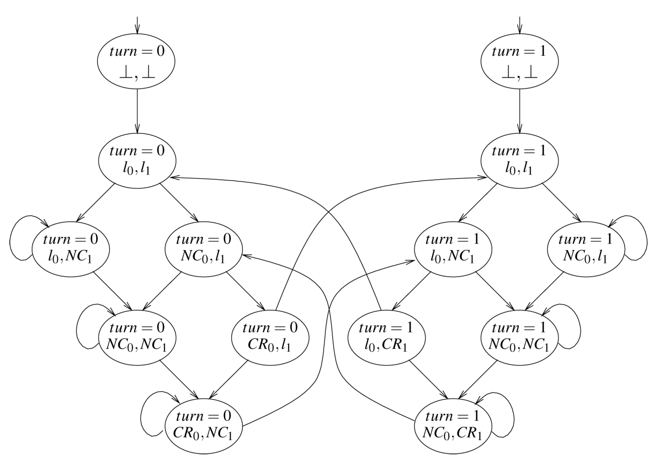
#### wait の例: 交互実行
以下のプログラムを考える
$$
\begin{aligned}
P_0 =& &P_1 = & \\
&l_{0};\text{while } true\text{ do} & &l_{1};\text{while } true\text{ do}\\
&\quad NC_{0}; wait(turn = 0); & &\quad NC_{1}; wait(turn = 1);\\
&\quad CR_{0}; turn := 1; & &\quad CR_{1}; turn := 0;\\
&\text{end while}; l_{0}' & &\text{end while}; l_{1}'\\
\end{aligned}
\begin{aligned}
P =\\
&m&\\
&\text{cobegin }P_0 \parallel P_1\text{ coend}&\\
&m'&\\
\end{aligned}\\
$$
クリプキ構造の図
translation procedure は
* Concurrent Processes の起動
$pc = m \wedge pc' = susp \wedge pc_0' = l_{0} \wedge pc_1' = l_{1}$
* thread 0 の処理
$\mathcal{C}(l_{0},P_0,l'_{0}) \wedge same(\{pc, pc_1\})$
* thread 1 の処理
$\mathcal{C}(l_{1},P_1,l'_{1}) \wedge same(\{pc, pc_0\})$
* Concurrent Processes のjoin
$pc = susp \wedge pc_0 = l_{0}' \wedge pc_1 = l_{1}' \wedge pc' = m' \wedge pc_0' = susp \wedge pc_1' = susp$
の$\vee$
ただし、
$$
\begin{aligned}
\mathcal{C}(l_{i},P_i,l'_{i}) =&
(pc_i = l_i \wedge pc_i' = NC_i \wedge turn'=turn)\\
\vee& (pc_i = NC_i \wedge turn \neq i \wedge pc_i' = NC_i \wedge turn'=turn)\\
\vee& (pc_i = NC_i \wedge turn = i \wedge pc_i' = CR_i \wedge turn'=turn)\\
\vee& (pc_i = CR_i \wedge pc_i' = l_i \wedge turn'=(turn+1)%2)\\
\end{aligned}
$$
二つのプロセスが同時にCRに入ることが無いことがわかる。
::: spoiler Q. starvation (どちらかのプロセスのCRが実行されない) が起こるパスは存在するか
存在する。
turn=1の状態で、プロセス0を実行し続ける場合に starvation が起こる。
プロセス0を実行し続ける場合は無いという主張をするのが後述の Fairness 。
:::
### Transition の粒度
model 上の処理の最小単位と、実装での処理の最小単位が一致していない場合、問題が起こることがある。
2つの命令
$$
\begin{aligned}
\alpha: &x = x + y\\
\beta: &y = y + x
\end{aligned}
$$
と、$\alpha,\beta$をより細かく分解した命令群
$$
\begin{aligned}
\alpha_0: &\text{load }R_1,x &\beta_0: &\text{load }R_2,y\\
\alpha_1: &\text{add }R_1,y &\beta_1: &\text{add }R_2,x\\
\alpha_2: &\text{store }R_1, x &\beta_2: &\text{store }R_2, y\\
\end{aligned}
$$
を考える。
初期状態が$x = 1 \wedge y = 2$とする。
αとβを並列に実行する。
このときの実行結果として考えられる値は
* αとβの粒度のとき
* ::: spoiler αβ
$x = 3 \wedge y = 5$
:::
* ::: spoiler βα
$x = 4 \wedge y = 3$
:::
* 細かい粒度のとき
* α0α1α2β0β1β2
$x = 3 \wedge y = 5$
* β0β1β2α0α1α2
$x = 4 \wedge y = 3$
* ::: spoiler α0β0α1β1α2β2
$x = 3 \wedge y = 3$
:::
#### 粒度が違うと困る例
* 実際のシステムがαとβの粒度だが、modelが細かい粒度のとき
* model上の方がより多くの状態に到達できてしまう
* liveness の証明に使えない
* 例えば、モデル上で$x = 3 \wedge y = 3$に到達するという結果が出ても、信頼できない
* 状態数が増えるので検査の時間計算量が増える
* 実際のシステムが細かい粒度だが、modelがαとβの粒度のとき
* 実際のシステムの方がより多くの状態に到達できてしまう
* エラー検出に使えない
* 例えば、モデル上で$x = 3 \wedge y = 3$にならないという結果が出ても、信頼できない
## Fairness
Concurrent Processes があるときにどのパスを実行するかは、実システム上では scheduler が決める。
scheduler は複雑なので、直接モデル化するのではなく、代わりに Fairness 制約を導入する。
Kripke structure $M = (S,S_0, R, AP, L, F)$
* $F \subseteq 2^{S}$: Fairness 制約
### Fairness 制約の定義
無限長パス$\pi$が Fairness 制約$F = \{F_1,F_2,\dots,F_n\}$を満たしているとは
$\forall F_i \in F,\quad \exists s \in F_i,\quad M, \pi \models GF s$
$F_1$に含まれている要素のどれかが無限にしばしば現れる、かつ
$F_2$に含まれている要素のどれかが無限にしばしば現れる、かつ
$\vdots$
$F_n$に含まれている要素のどれかが無限にしばしば現れる
#### スケジューリングによる starvation を回避する Fairness 制約
直前に実行されたプロセスIDを保存する変数を用意する。
$\sigma_i$を直前に実行されたプロセスが i のときに true になる変数、とする。
$$
\begin{aligned}
F_i &= (\sigma_i \vee pc_i = susp)\\
F &= \{F_1, \dots, F_n\}
\end{aligned}
$$
各プロセスが、
* 実行されていない
* 無限にしばしば実行される
のどちらかであれば良い。
 Sign in with Wallet
Connect another wallet
Sign in with Wallet
Connect another wallet