# Reproducing FDA: Fourier Domain Adaptation for Semantic Segmentation

:::success
The code for this reproduction is available on [GitHub](https://github.com/crnh/FDA).
:::

[TOC]

## Introduction

### Semantic segmentation
Semantic segmentation is a type of image segmentation where every pixel is assigned a certain label, without differentiating between multiple objects of the same class [^nanonets]. We will look at using semantic segmentation for the use of self-driving cars, where a pixel level understanding of the surrounding is necessary for, for instance, identifying driving lanes, other cars and pedestrians.

![**Fig. 1** - Example of semantic segmentation in the Cityscapes dataset, where the different colours represent different lables given to specific pixels. [^acdcpaper]](https://i.imgur.com/8ywWgoN.png)
**Fig. 1** - Example of semantic segmentation in the Cityscapes dataset, where the different colours represent different lables given to specific pixels. [^acdcpaper]

Semantic segmentation methods for self-driving cars generally use deep neural networks (DNN) trained on datasets such as Cityscapes [^fdapaper][^cityscapes]. These datasets consist of manually labeled photographs taken while driving around in urban areas. Since this manual labeling is very time-consuming, there is a need for a way to train the DNN on already labeled synthetic data, such as images taken from the video game GTA5, which produces inherently labeled images. The downside of doing this is that DNN's trained on synthetic data tend to perform poorly on real life images [^fdapaper]. A way to overcome this problem is by using domain adaptation.

![**Fig. 2** - Example of semantic segmentation in the GTA5 dataset. [^gta5]](https://i.imgur.com/FpE29uy.png)
**Fig. 2** - Example of semantic segmentation in the GTA5 dataset. [^gta5]

### Fourier Domain adaptation

The goal of domain adaptation is to train a neural network on one dataset (source domain) and secure a good performance on another dataset (target domain), by for instance making the source set look more like the target set [^domain-adaptation]. Most of the times it is the case that it is very easy to generate labeled source data, while it is much more time-consuming to generate labeled target data, such as when using GTA5 [^gta5] as source data and Cityscapes as target data. Therefore, doing this allows for having more labeled data available, while it is still in the "style" of the target images.

Different types of domain adaptation exist, most of which use complicated adversarial neural networks. These networks work by training on the source data, while using a second network to generalize to the target data. However Yang et al. [^fdapaper] introduce a relatively simple method called Fourier Domain Adaptation (FDA). This method works by replacing the center part of the Fourier domain (FD) amplitude of the source image with the center part of the FD amplitude of the target image, as depicted in Figure 3. By taking the inverse Fast Fourier Transform (FFT) of the source image, you end up with a source image in which the low frequencies are modified to better match the target image.

**Fig. 3** - Visualization of the FDA algorithm. The green square indicates the part of the source FD amplitude that is being replaced by the corresponding target FD amplitude, where $\beta$ is the height of the square relative to the height of the image. In this image, the value of $\beta$ is exaggerated.

The rationale of this method is that low frequency amplitude can vary a lot between synthetic and real life images, causing a network trained on synthetic data to perform poorly on real life data. By replacing the low frequency amplitude of the synthetic data with that of the real life data, the low frequency amplitude is changed without affecting the semantic information. In other words, whether something is seen as a car, pedestrian or streetlight should not depend on, for instance, the illumination of the image [^fdapaper]. FDA can help to make sure that the network is not sensitive to these kind of changes.

### Fourier Domain

To understand why we would want to copy the amplitude part of the target image, let’s consider what the phase and amplitude of the Fourier domain say about an image.
As you may know the Fourier domain shows us with which sines and cosines (or complex exponentials if you want to be fancy) we can construct our image.
As these sines and cosines represent waves we know that they can be described by their phase and amplitude. The figure below illustrates what the phase and amplitude of these wave contribute to.

**Fig. 4** - This figure shows the inverse Fourier transform of both the amplitude and the phase part of the Fourier domain. From this figure it is clear to see that the phase part of the Fourier domain gives the structure of the image and the amplitude part only weights which waves should be more prominent than others.

So, now our Fourier theory is refreshed, we can start whether the technique proposed in [^fdapaper] makes sense. The authors propose to use a square region to copy the target amplitude, but they don't motivate this decision. We think that a square shape is not the most logical choice, this is because the frequencies increase when moving radially away from the origin. So when taking a square region you are selecting a variable range of frequencies, since the corners of the square contain higher frequencies. We therefore hypothesize that a radially symmetric region is better aligned with the structure of Fourier space, and may perform better than a square. We tested our hypothesis by training the provided model but with two different regions, one circular and the other Gaussian weighted.

### Research goal

Our goal is to reproduce the results of the FDA paper by Yang et al. [^fdapaper] for the GTA5 source data and Cityscapes target data for $\beta$ = 0.01, using a DeepLabv2[^deeplab] backbone. Furthermore, to investigate the effect of the shape of the area of the low frequency FD amplitude that is being replaced, our goal is to create a circular "kernel" for this, instead of the square kernel used in the FDA paper. Furthermore, we also want to create a Gaussian weighted full image kernel for the FDA and compare the results of both of these kernels with the results of the original square kernel.

## Experiments

As a starting point for our reproduction, we used the code provided by the authors[^fdacode]. We made a few modifications to the existing code:

* In order to get the code working with the CUDA version installed in Google Colab and our Google Cloud VM, it was necessary to port the code to a newer PyTorch version (1.10). We had to update the code for the changed `torch.fft` module (for the Fourier transforms in the FDA step) and the way in which complex numbers are handled. We inspected the images generated with our adjusted FDA code, and found no evidence for this change to impact our results.
* Some extra code was added to the training loop, to allow for storing the losses and other metrics in Tensorboard. Additionally, we added some code to calculate the mIoU during training, using [`sklearn.metrics.jaccard_score`](https://scikit-learn.org/stable/modules/generated/sklearn.metrics.jaccard_score.html).
* The ability to use different mask shapes (square, circle and Gaussian) was added to the FDA code.
* An optional downsampling step was added to the data loading procedure, but this has not been used in our final experiments.

All experiments were performed on an Nvidia Tesla K80 GPU in a Google Compute virtual machine, with 4 vCPUs and 26 GB of memory. When downloading the GTA5 dataset, one image (`20106.png`) was corrupted, and we deliberately decided to not download the dataset again, but leave this image out instead. Therefore, the GTA5 dataset used in our experiments contained 22499 images.

### FDA shape modification

As mentioned in the introduction, in our experiments we aim to compare the square shape a introduced in the paper to our implementation of both a circular and Gaussian shaped region. In this section we will examine how we constructed the masks.

**Fig. 5** - This figure shows the three shapes that we used for the Fourier domain adaptation: square, circular and Gaussian with $\beta =0.09$.

We thought about what would be the most fair way to compare the different shapes. For example, a Gaussian is more spread out than a circle, so just setting the standard deviation of the Gaussian equal to the diameter of the circle was a little too crude of a way of doing it. We finally decided that we would keep the area under the masks equal between the shapes. In this way the same amount of “information” is copied from the source to the target domain, irrespective of the region shape. We measured this amount of information in terms of the "volume" of replaced pixels. For the square and circle this meant that we just multiplied their area with one as they were binary masks and the Gaussian was normalized and then multiplied with the desired volume.

We thus also needed to convert the $\beta$ parameter to a metric useful for the shape in question, we therefore derived the following relations. So, we needed to convert the $\beta$ parameter in the paper so that the volume under the curve was equal.
$$
\begin{aligned}
\mathrm{Square}: A = \beta ^2
\end{aligned}
$$
$$
\begin{aligned}
\mathrm{Circle}: r = \frac{ \beta }{ \sqrt{\pi} }
\end{aligned}
$$
$$
\begin{aligned}
\mathrm{Gaussian}: \sigma^2 = \frac{ \beta^2 }{ 2 \pi }
\end{aligned}
$$

Here we will go in to more detail on how we constructed the Gaussian mask, since the implementation is not trivial as with the square and circle. In effect we used two masks. The first mask is a 2D Gaussian and the second one the inverse of the Gaussian. These mask are shown in figure 6.

**Fig. 6** - This figure shows the cross-section of the Gaussian mask and the inverse Gaussian mask.

We applied these masks in the following way: firstly we multiply the inverse mask with the amplitude of the source image, to “create a hole” where our target amplitude could fit in to. Secondly, we multiply the target amplitude with the Gaussian mask. And finally, we add up the result of the mask target and source, to arrive at the final result.

### Training Runs

To keep the experiments within our time and financial budgets, we had to use a shorter training regime than used in the original paper. This was the main concern when deciding what runs to perform. The experiments we performed are summarized in table 1.

Here we will shortly describe what the training procedure looks like. In each iteration, we randomly draw an image from the GTAV dataset and use this images as source image. Furthermore, we randomly select an image from the Cityscapes dataset. The source image is altered by the FDA, and a forward and backward pass are performed using the modified image. After this forward pass, another forward pass is done using the target image. The loss of this image is included in the overall loss function in a special way; for details we refer to [^fdapaper]. During each iteration, losses are calculated and stored for both the source image and the target image.

***Table 1** Summary of the different experiments. All experiments used a batch size of 1 and a learning rate of $2.5 \times 10 ^{-4}$; these are the defaults used in [^fdapaper]. The first row contains the parameters used in the paper for the result we try to reproduce.*

| Experiment | Iterations | # source samples | # target samples | Beta | FDA shape |
| ---------------------- | ----------:| ----------------:| ----------------:| ----:| --------- |
| Article | 150000 | 22499 | 2975 | 0.01 | square |
| Reproduction | 38000 | 22499 | 2975 | 0.01 | square |
| Square | 12500 | 12500 | 2975 | 0.09 | square |
| Circle | 12500 | 12500 | 2975 | 0.09 | circle |
| Gaussian | 12500 | 12500 | 2975 | 0.09 | gaussian |
| Gaussian long training | 38000 | 22499 | 2975 | 0.01 | gaussian |

We aimed to reproduce the paper as closely as possible so we tried to keep most hyperparameters of the model constant like the learning rate ($2.5 \times 10 ^{-4}$) and the batch size ($1$).

The first experiment we performed was a reproduction experiment on the full GTA5 dataset as source domain, and the full Cityscapes dataset as target domain. Although the number of iterations is decreased with respect to the experiments in the paper, every image is used at least once during our training procedure.

For the experiments with different FDA kernels, we used a shorter training regime (12500 iterations). Only 50% of the GTA5 dataset was used as source domain, and the full Cityscapes dataset as target domain. The same seed was used for all experiments, so the order in which the images were fed to the network was the same for all experiments. We chose to used $\beta = 0.09$ for these experiments as the paper reported the best result for a square region for this value.

In these experiments the Gaussian performed marginally better (see table 2). Therefore, we wanted to know if this result was also reproducible with a longer training procedure. So, we performed a run with 38000 iterations, the same as the first reproduction training. Here we used $\beta= 0.01$ for a fair comparison with the first reproduction training.

The models produced by the experiments were all evaluated on the validation set of CityScapes[^cityscapes]. In the next section, we report the Intersection over Union (IoU) for each class, and the mean IoU (mIoU) for every experiment.

## Results

The performances of all the experiments performed are given in Table 2. Let's first draw our attention to the difference between our reproduction and the performance given in the article. First of all, we see that our reproduction performs worse than the article on almost all labels. This can be expected since, although we use the same number of source and target samples, we only use 1/4 of the number of iterations. However, it is clear that the performances for different labels are correlated since the reproduction is pretty consistently a bit lower than the article performance.

***Table 2** Results for the performance of the different experiments performed, for all labels separately (IoU) and for the mean intersection over union (mIoU). The performance given in the FDA paper is given under Article. Relevant parameter values for all experiments are listed in table 1.*

| Experiment | road | sidewalk | building | wall | fence | pole | light | sign | vegetation | terrain | sky | person | rider | car | truck | bus | train | motorcycle | bicycle | **mIoU** |
| --------------------------- | -----:| --------:| --------:| -----:| -----:| -----:| -----:| -----:| ----------:| -------:| -----:| ------:| -----:| -----:| -----:| -----:| -----:| ----------:| -------:| ---------:|
| Article | 88.8 | 35.4 | 80.5 | 24.0 | 24.9 | 31.3 | 34.9 | 32.0 | 82.6 | 35.6 | 74.4 | 59.4 | 31.0 | 81.7 | 29.3 | 47.1 | 1.2 | 21.1 | 32.3 | **44.61** |
| Reproduction | 86.15 | 35.0 | 78.82 | 18.8 | 23.1 | 31.1 | 31.84 | 25.61 | 82.66 | 34.81 | 71.66 | 58.89 | 25.66 | 76.09 | 22.63 | 35.42 | 1.43 | 24.17 | 30.73 | **41.82** |
| Gaussian long training | 82.54 | 32.74 | 78.75 | 16.83 | 25.86 | 31.08 | 30.36 | 25.85 | 82.04 | 37.23 | 74.43 | 60.19 | 24.17 | 70.61 | 30.89 | 41.15 | 0.08 | 20.83 | 17.14 | **41.2** |
| Square | 80.45 | 34.11 | 77.52 | 15.18 | 17.33 | 27.16 | 26.93 | 22.78 | 78.53 | 36.74 | 68.88 | 58.04 | 21.16 | 79.79 | 19.04 | 38.24 | 1.06 | 19.77 | 31.46 | **39.69** |
| Circle | 75.48 | 31.6 | 77.54 | 10.89 | 20.44 | 27.14 | 27.61 | 24.61 | 81.24 | 37.07 | 73.83 | 58.22 | 22.58 | 81.11 | 18.32 | 44.95 | 1.74 | 15.78 | 15.8 | **39.26** |
| Gaussian | 81.2 | 30.89 | 77.8 | 21.23 | 19.42 | 28.2 | 27.37 | 23.07 | 80.29 | 39.22 | 71.05 | 58.52 | 21.88 | 81.15 | 20.78 | 42.42 | 1.31 | 18.33 | 24.32 | **40.45** |

When looking at the performances of a square, circular and Gaussian FDA kernel, we find that the Gaussian kernel slightly outperforms the other kernels, as it has a slightly higher mean intersection over union (mIoU). However, since the difference in performance is so low, it is difficult to draw conclusions from these experiments. Lastly, when comparing the Gaussian long training with our reproduction (since these use the same number of iterations), we see that it overall performs slightly worse than the reproduction, but again not significantly. This shows that, although with the shorter training the Gaussian performed best, we cannot conclude that it performs better than the square FDA kernel.

To see the effect of the different FDA kernel shapes, examples of the adapted source images can be seen in Figure 7. It may be clear that all three images show some weird artefacts in the form of spots, just like in the adapted source image in Figure 3. When going from square to circle to Gaussian, the artefacts appear to be more blurred and less periodic, while the dark spots seem to align in all three figures. This can be explained by the fact that the Gaussian kernel does not have a clear cut off, while the others do, which can be the reason why the artefacts are less periodic.

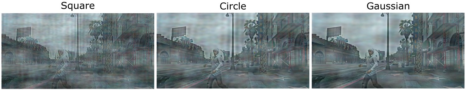
**Fig. 7** - Comparison of the adapted source images for different FDA kernel shapes.

Example results from the segmented target images for using the networks described in Table 2 are given in Figure 8. Here, the segmentation performed by a pretrained network provided by Yang et al. [^fdapaper] is also included. However, the pretrained network uses Multi Band Transfer (meaning it averages results obtained using multiple values of $\beta$), which results in a higher accuracy than the result we aim to reproduce. It shouldn't therefore be directly compared to our reproduction result.
Additionally, in the figure we can see that the all the reproductions we made have the same overall structure and include the same labels. However, the segmentations produced by models trained with fewer iterations contain more artefacts, for instance on the road and on the edges between street and sidewalk. This shows that additional training time would be beneficial. When comparing the different FDA shapes, we can see that the Gaussian produces more continuous label boundaries, but this difference is not large.

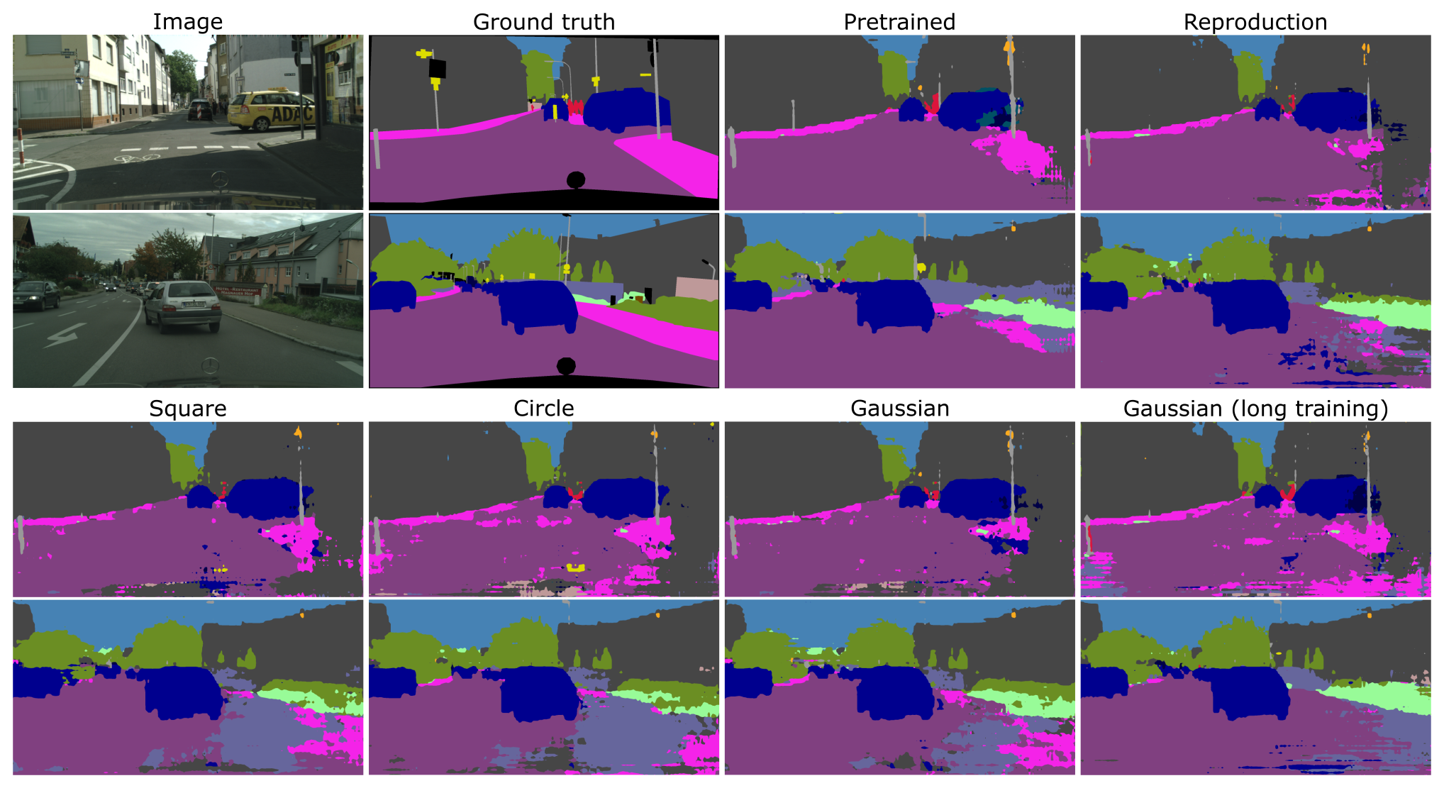
**Fig. 8** - Example results for 2 segmented target images. Top row: original image, ground truth segmentation, segmentation from the pretrained network (max. 150000 iterations) provided by the authors, and segmentation from our reproduction using 38000 iterations. Bottom row: segmentations from networks trained using a circular, square or Gaussian FDA kernel, with 12500 iterations. The last result is for a Gaussian kernel and 38000 iterations. The segmentations produced by networks trained with fewer iterations show relatively many artefacts. Most artefacts occur on the road and on the edge between street and sidewalk. For the three different FDA shapes (bottom row), the Gaussian contains the smallest amount of artefacts, but this is not the case for the Gaussian trained for 38000 iterations.

The source and target training loss and accuracy for the three different FDA kernels (Square, Circle and Gaussian) are given in Figure 9. In this figure, it is interesting that the training loss for the circle FDA is lower (and the accuracy higher) than for the square FDA. However, on the validation set the accuracy for circle FDA was lower. The source and target training loss and accuracy for the square and Gaussian kernels (Reproduction and Gaussian long training) with 38000 iterations are given in Figure 10.

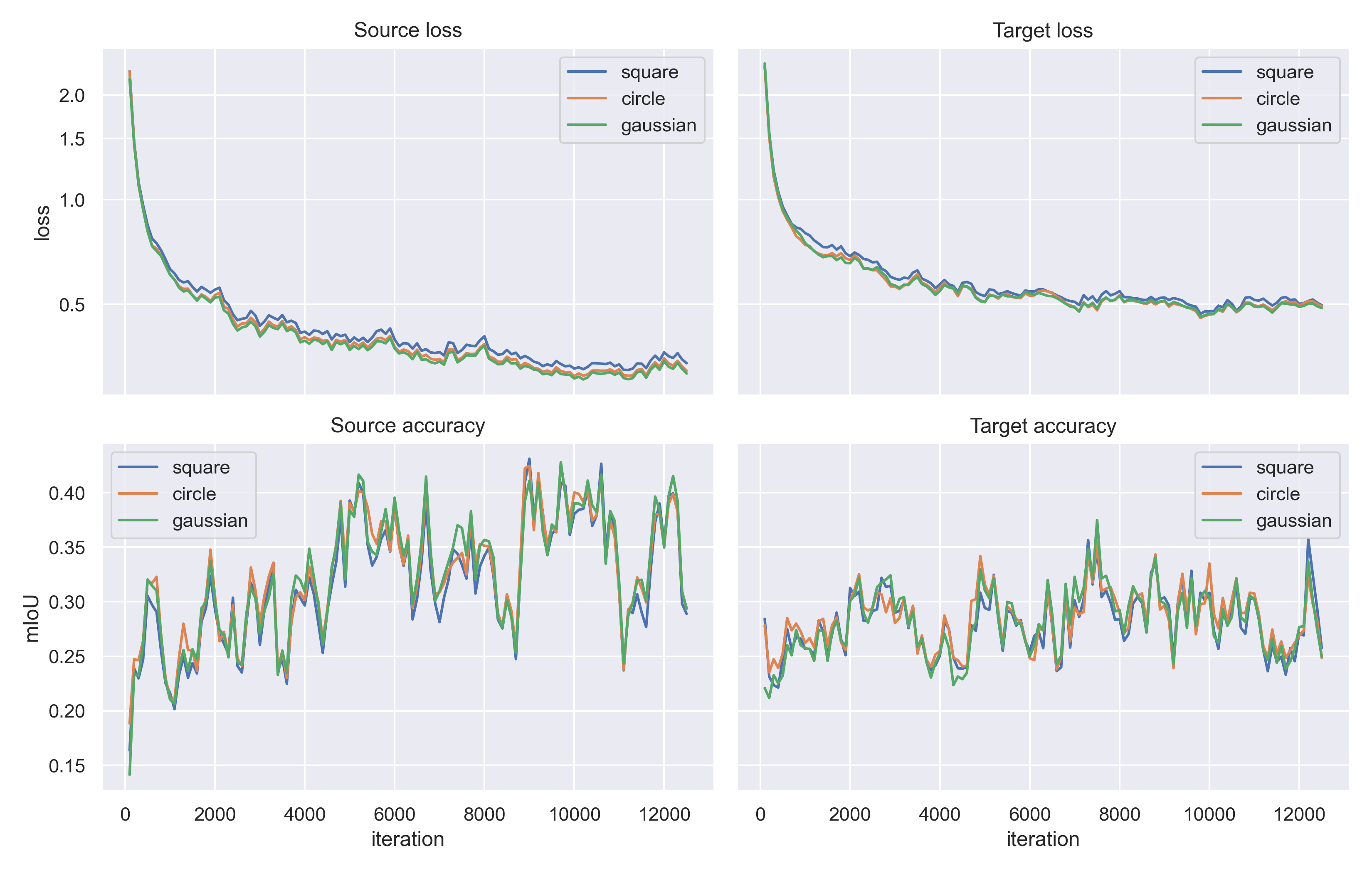
**Fig. 9** - Training losses and accuracies on the source and target datasets, for the three different FDA kernels. Both the circle and the Gaussian losses are lower than the square loss, but only the Gaussian kernel yields a higher mIoU. All methods perform consistently better on source data than on target data. The accuracies show large jumps, which is probably caused by the small batch size of 1 image. The curves were smoothed a bit in order to keep the figure readable.

**Fig. 10** - Training loss and mIoU on the source and target datasets, for the reproduction experiment (38000 iterations). The experiment was repeated for square and gaussian FDA kernels. The accuracy curves were smoothed a bit in order to keep the figure readable. Unfortunately, the authors of the FDA paper did not provide the training losses, so we are unable to compare our losses with the original implementation.

## Discussion

### Reproducibility with fewer iterations

One of our goals was to reproduce the results of the FDA paper by Yang et al.[^fdapaper] We did not succeed in this since we got a lower performance than given in the paper. However, we used only a quarter of the iterations described in the paper (38000 instead of 150000), which could be the reason of our lower performance. This raises the question of how much can be said about the reproducibility of this paper based on our findings. After 1/4th of the iterations, the accuracy has already come close to the values in the paper and appears to be still slowly increasing. It is therefore likely that after running the full amount of iterations, the accuracies listed in the paper can be reproduced. In order to test this, we suggest to rerun the experiment with the same amount of iterations used in the paper.

### Normalisation of kernels

In our experiments, we normalized the FDA kernels of different shapes so that all have the same volume. In case of the square and circular kernels, the volume is equal to the area, while for the Gaussian, it is the 2D integral over the curve. This approach was chosen to make sure that the same amount of information in the Fourier domain is transferred, however, one can wonder whether this is the case. Since the amplitude of the Fourier domain varies a lot, another way of normalizing could be to normalize to the amplitude of the Fourier domain inside the kernel. In this way, the same amount of amplitude is always transferred, making the size of the kernel depend on the image. In order to find the optimal kernel shape and size, a parameter search should be performed where different $\beta$'s for different kernel shapes should be tested. It could be that the optimal value of $\beta$ differs for each kernel.

### Segmentation of car hoods

An interesting thing to note in Figure 8 is that none of the networks are able to segment the car hood of the car from where the photograph is made, as is given in black in the ground truth. The black label represents "nothing", which is used for objects that don't belong to one of the classes, for instance mirrors and the back of signs. This can be explained by the fact that the network is not able to apply the "nothing" class as a design choice. This makes sense since it would be perhaps be weird to give the network the option to just say an object is "nothing". It is probably better to force the network to give it's best try. It can be observed in Figure 8 that for the shorter trained networks, the car hood is mostly given the label of "building", while for the longer trained networks it is mostly "car" or "road",

## Conclusion

During this reproduction we have shown that we could get relatively close to the values reported in the paper. However, our experiments on the effect of FDA shapes on the segmentation performs show no indication that Gaussian or circular shapes outperform the square baseline. This may be due to the relatively low number of iterations in our experiments, where it could be the case that small differences only reveal themselves near the point where the training converges.
Thus, there still remain open questions that are interesting to look into, such as: does a longer training result in significant differences between FDA kernel shapes? And would a more extensive parameter search result in better performance than on the circular and Gaussian FDA kernel?

[^fdapaper]: Y. Yang and S. Soatto, “FDA: Fourier Domain Adaptation for Semantic Segmentation,” arXiv:2004.05498 [cs], Apr. 2020, Accessed: Feb. 28, 2022. [Online]. Available: http://arxiv.org/abs/2004.05498

[^fdacode]: YanchaoYang, FDA: Fourier Domain Adaptation for Semantic Segmentation. 2022. Accessed: Apr. 14, 2022. [Online]. Available: https://github.com/YanchaoYang/FDA

[^deeplab]: L.-C. Chen, G. Papandreou, I. Kokkinos, K. Murphy, and A. L. Yuille, “DeepLab: Semantic Image Segmentation with Deep Convolutional Nets, Atrous Convolution, and Fully Connected CRFs,” arXiv:1606.00915 [cs], May 2017, Accessed: Apr. 14, 2022. [Online]. Available: http://arxiv.org/abs/1606.00915

[^acdcpaper]: C. Sakaridis, D. Dai and L. Van Gool, “ACDC: The Adverse Conditions Dataset with Correspondences for Semantic Driving Scene Understanding,” arXiv:2104.13395 [cs.CV], 2021, Accessed: Apr. 12, 2022. [Online]. Available: https://arxiv.org/abs/2104.13395

[^cityscapes]: M. Cordts et al., “The Cityscapes Dataset for Semantic Urban Scene Understanding,” Apr. 2016, doi: 10.48550/arXiv.1604.01685.

[^gta5]: S. R. Richter, V. Vineet, S. Roth, and V. Koltun, “Playing for Data: Ground Truth from Computer Games,” Aug. 2016, doi: 10.48550/arXiv.1608.02192.

[^nanonets]: “A 2021 guide to Semantic Segmentation,” AI & Machine Learning Blog, May 19, 2021. https://nanonets.com/blog/semantic-image-segmentation-2020/ (accessed Apr. 07, 2022).

[^domain-adaptation]: “Understanding Domain Adaptation. Learn how to design a deep learning… | by Harsh Maheshwari | Towards Data Science.” https://towardsdatascience.com/understanding-domain-adaptation-5baa723ac71f (accessed Apr. 07, 2022).

[FDA paper]: http://arxiv.org/abs/2004.05498 "Y. Yang and S. Soatto, “FDA: Fourier Domain Adaptation for Semantic Segmentation,” arXiv:2004.05498 [cs], Apr. 2020, Accessed: Feb. 28, 2022. [Online]. Available: http://arxiv.org/abs/2004.05498"
[2]: https://github.com/YanchaoYang/FDA "Original code provided by the authors of the FDA paper"