# WEEK 5 (14-18/12/20)
## What is Machine Learning? (Mon, 14/12/20)
### **ML algorithms**

* Build a ==mathematical model== based on sample data, known as "training data"
* Make ==predictions or decisions== without being explicitly programmed to do so
* Can spot patterns and make predictions about future events

---
### Applications of ML
* **Predicting**: stock price, fraudulent transaction, profuct sales, apartment rents, ...
* **Recommendation systems**
* **Natural language processing (NLP)**: Answering questions; speech recognition; summarizing documents,...
* **Computer vision**: image captioning; reading traffic signs; locating pedestrians and vehicles in autonomous vehicles
* **Image generation**: Colorizing images; increasing image resolution; removing noise from images
* **Medicine**: Finding anomalies in radiology images, including CT, MRI, and X-ray images; predict skin-cancer with near-human accuracy

---
### Types of Machine Learning

**==Supervised Learning==**
* To learn a model from ==labeled training data==
* The learned model can **make predictions** about ==unseen data==
* “Supervised”: the label/output of your training data is already known

**Types of function**:
* Neural network
* Decision tree
* Other types of classifiers

==**Hypothesis class 𝐻**==: a set of possible ML function

==**No Free Lunch Theorem**==
Every successful machine learning algorithm has to **==make assumptions==** about the dataset/distribution 𝑃
---> There is no perfect algorithm for all problems

**==Loss Function==**: evaluate the model on our training set to tells us how bad it is.
---> The higher the loss, the worst it is. A loss of zero means it makes perfect predictions.
Example: MSE

(y hat: output of model)
---

### **==Overfitting and Underfitting==**
**Generalization**: ability to perform well on previously unobserved inputs

**Split** your dataset 𝐷 into **three** ==subsets==:

**ASSUMPTION**:
* training set and test set are ==identically distributed==
* samples in each dataset are ==independent== from each other

**Why do we need 𝐷𝑉𝐴 ?**

* In the training process, the model needs to be ==validated== on 𝐷𝑉𝐴 .
* If the error is too large, the model will get revised based on 𝐷𝑇𝑅 , and validate again on 𝐷𝑉𝐴 .
* This process will keep going back and forth until it gives ==low loss== on 𝐷𝑉𝐴 .

==**Overfitting**==: big deviation between train error and validation error, perform badly with unseen data (low train error, high validation error)

==**Underfitting**==: model makes high error on **both** trainning and validating set

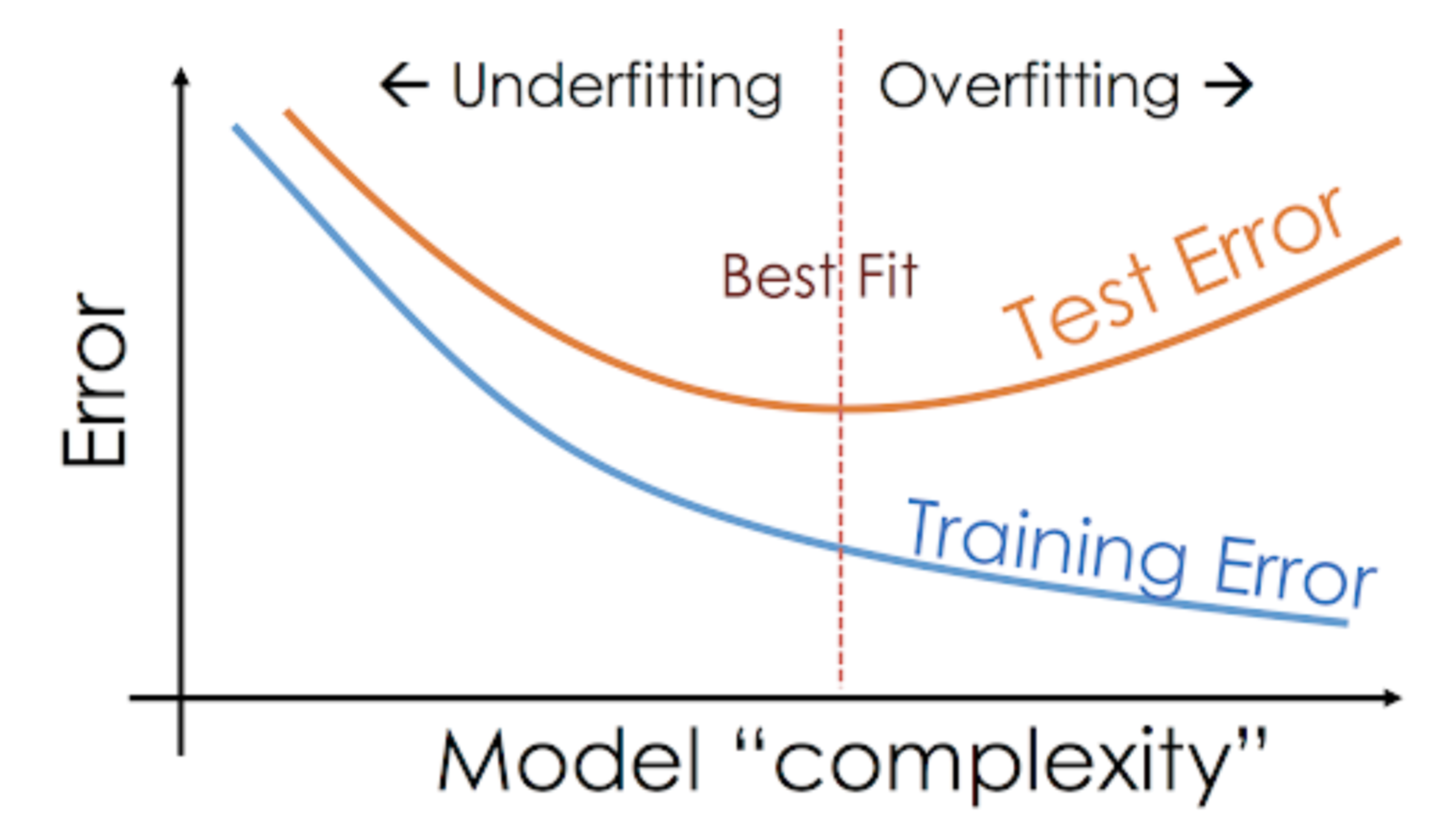
==**Altering capacity**==
Models with:
* ==High== capacity: over memorized propertise of training, perform badly on the test set ---> overfit
* ==Low== capacity: struggle on trainin set, high error on training set

---

### **==Limitations of Machine Learning==**
* Must have **LABELLED** data
* ML can only make **PREDICTIONS**, not recommended actions
* Bias data and Feedback loops danger

### Probability
**Random variables**: a function that maps outcomes of random experiments to a set of properties (numbers)

**Probability distribution function**: a function that measures the probability that a particular outcome or set of outcomes will occur

**==BASICS==**
* The **sample space Ω** is a ==fixed== set of all possible outcomes.
* The probability 𝑃(𝐴) measures the probability that the event 𝐴 will occur.
* Two events 𝐴 and 𝐵 are **dependent** if knowing something about whether 𝐴 happens gives us information about whether 𝐵 happens(and vice versa). Otherwise, they are **independent**


**==Expected value==**: the sum of the possible outcomes ==weighted== by their probability (**long run average**)
* Discrete x:

* Continuous x:

**==Distribution==**
**Unique nonnegative functions**:
* 𝑓(𝑥) (probability density function PDF)
* 𝐹(𝑥) (cumulative distribution function CDF)

* If x is **discrete**, 𝑓(𝑥) is called probability mass function PMF:

==**Common discrete distributions:**==
* Bernoulli (where 0≤𝑝≤1 )

* Binomial(n, p) (where 0≤𝑝≤1)

==**Common continuous distributions:**==
* Uniform(a,b) (where a < b)

*
( 𝜇 , 𝜎2 )

### **==Central limit theorem==**
The sample mean of a sufficiently large number of i.i.d. random variables is approximately ==normally distributed==. The **larger** the sample, the **better** the approximation.

---

## Maths in ML (Tue, 15/12/20)
### Linear Algebra
#### **==Vector==**
A ==vector== represents the magnitude and direction of potential change to a point
Vectors are elements of 𝑅𝑛 (lists of n real number)
==**Scalar multiplication**== (increase/decrease magnitude of vector)

==**Addition**==

==**Unit vector**==
Unit vectors are vectors of length 1

==**Dot product**==
!!! DOT PRODUCT of vector a and b is:
* positive when they point at 'similar' direction. Bigger = more similar
* equals 0 when they are perpendicular
* negative when they are at dissimilar directions. Smaller(more negative)=more dissimilar
---> Drawback: there is no scale must compare with something

**==Cosine similarity==**: calculating cosine of the angle 𝜙 between two vectors
The resulting similarity is **between -1 and 1**:

**−1: exactly opposite** (pointing in the opposite direction)
between -1 and 0: intermediate dissimilarity.
0: **orthogonal**
between 0 and 1: intermediate similarity
**1: exactly the same** (pointing in the same direction)

Dot product properties:

**==Hadamard product (Element-wise multiplication)==**
Dot returns a **scalar** (1 single element)!!!
Element-wise multiplication returns a **vector** with the same dimension !!

#### **==Matrix==**
A matrix is a two-dimensional rectangular array of numbers

**==Matrix operations (element-wise)**==
1. ==Broadcasting==: the matrix of the smaller shape is expanded to match the matrix of the bigger shape

#### ==**Calculus**==
The derivative measures the slope of the tangent line.

## Linear Regression (Wed, 16/12/20)
Linear Regression:
* supervised machine learning algorithm
* solves a regression (predict infinite amount of things) problem
* Input: vector 𝑥∈𝑅𝑛
* Output: scalar 𝑦∈𝑅 .
* The value that our model predicts y is called 𝑦̂ , which is defined as:
where w and b are ==parameters==
w= vector of coefficients (weights)
b= intercept

**==FIND w,b SO THAT L(w,b) IS MINIMIZED==**

==TERMINOLOGY==
x=independent variable (aka features)
y=dependent variable (what we have to predict)
weight=slope (aka coefficient weights)
bias=y-intercept

==**Loss Function**== (MSE)
MSE: tells how good the function is at making predictions for a given set of parameters
---> ==SLOPE== of curve tells the direction we should ==update our weights== to make the model more accurate

FOR SIMPLE LINEAR EQUATION:

==**Gradient Descent**==
---> To ==minimize== MSE, calculate the gradient of our loss function with respect to our weight and bias

#### ==**Mulitple linear regression**==

## Logistic Regression (Thu, 17/12/20)

### **==Logistic regression==** (solve classification problems)

#### **==Sigmoid function==**
A sigmoid function placed as the last layer of a machine learning model can serve to ==convert== the model's output into a ==probability score==, which can be easier to work with and interpret.

#### ==**Loss function**==(cost function)
also called **==Binary cross entropy==**

==**Gradient descent**==
* **Forward propagation**

* **Backward propagation**

--->**==Sklearn==**
* **.fit** : do gradient descent behind the scene- look for coefficient and intercept

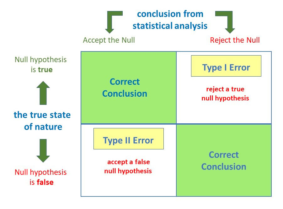
==**Type 1 and type 2 error**==
==Type 1 error== is also known as ==False Positive==, or FP (predict Positive, but actual label is Negative)

==Type 2 error== is also known as ==False Negative==, or FN (predict Negative, but actual label is Positive)

## Sentiment Analysis with Logistic Regression (Fri, 18/12/20)

count.fit_transform: prepare data
### **==Natural language processing==** (NLP)

### **==Bags of words==**
Count ==frequency== of each word, biggest problem- ignore the order of the words in a sentence ---> cannot understand the meaning.
Sparse matrix: That sparse matrices contain mostly zero values and are distinct from dense matrices.

==Term frequencies==
TF = (# occurrences of term t in document) / (# of words in documents)

### ==**Frequency-inverse document frequency (TF-IDF)**==
==Stop words== are words that are filtered out before or after the natural language data (text) are processed ("this", "a", "is")
---> high value of TF-IDF for important & informative words (NOT stop words)

* ==**Stemming**==: transforming different tenses of a word to 1 tense by getting rid of the ending part
eg, performing ---> perform

* ==**Lemmatization**==: default for this is noun (run very slow)

==Tokenize==: break down sentence into words

==**Pipeline**==