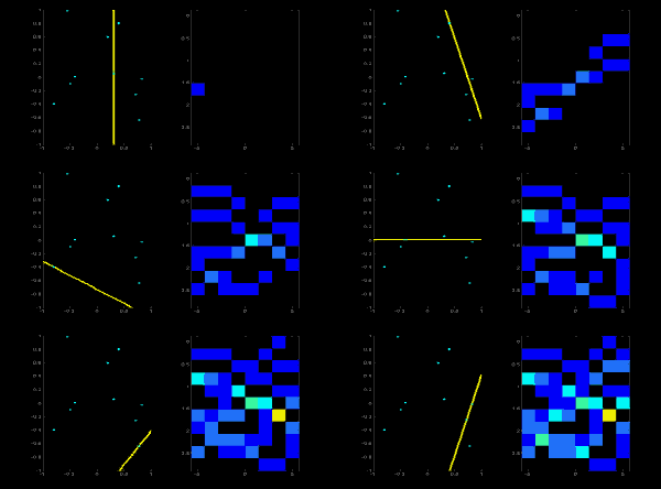
# HoughSpace

Explaing *Hough-Transform* for *line-space* and *curve-space*.

## 1. Hough transform for line

### 1.1 x-y Space
$f(x,y)$ => $y = ax + b$

which

* $a$: slope
* $b$: intercept

if we fixed $a = 0.5, b= 4.5$ , then

chart of $y = 0.5x + 4.5$ seems


(x,y) -> variable

(a,b) -> fixed

-> slope and intercept are fixed

-> fill **points**(Xn, Yn) inside the line bewteen the slope and the intercept

Summery:
Fixed **(a,b)**, you will get infinity **points** in the line

### 1.2 a-b Space

$g(a,b)$ => $b = -ax + y$

if we fixed $x = 0.5, y = 4.5$ , then

$b = -0.5a + 4.5$ , and

chart of $b = -0.5a + 4.5$ seems:


(slope = $-a/b$ = $tan($$\theta$$))$

(x,y) -> fixed

(a,b) -> variable

-> slope and intercept are mutable

-> fill(Rotate) **lines** where central point(strat point) fixed on (an,bn)

Summery:
Fixed **(x,y)**, you will get infinity **lines** on the point

### 1.3 Represent a-b Space with r-$\theta$ Space <br> aka Hough linear space

$h(r,$$\theta$$)$ => $r$ = $xcos($$\theta$$) + ysin($$\theta$$)$


if we mapping a linear eq.(a-b space) to r-$\theta$ space


### 1.4 Accumulator with r-$\theta$ Space



### 1.5 Summary: Flow of Hough Algorithm r-$\theta$ Space

1. Filtering input data or image(not found in paper)
2. Calculating (r,$\theta$) for each point which stayed after step 1
3. Choosing (r,$\theta$) with threshold
4. Rebuilding line with (r,$\theta$)

### 1.6 Naive implementation (python)

https://github.com/curly-wei/small-program/blob/master/python_training/hough/hough-line-space-2D.py


### 1.7 Or refer to here

https://docs.opencv.org/2.4/doc/tutorials/imgproc/imgtrans/hough_lines/hough_lines.html

## 2. Hough transform for curve

### 2.1 Explain

The curve of eq. in x-y space, we can express with

$(x-h)^2 + (y-k)^2 = r^2 ...eq.1$


If a center point of circuit at $(0,0)$,

then we can assume:

$h = r cos(t)$

$k = r sin(t)$

Substituting $r cos(t)$ and $r sin(t)$ into $(h,k)$ of $eq.1$,

we'll obtain:

$(x-r cos(t))^2 + (y-r sin(t))^2 = r^2 ...eq.2$

Arranging $eq.2$:

$r = \frac{1}{2} \frac{x^2 + y^2}{x cos(t) + y sin(t)} ...eq.3$

[Demo](https://www.youtube.com/watch?v=Ltqt24SQQoI):


Now,

assume that we have the eqution of circit $(x-0)^2 + (y-0)^2 = 5^2 ...eq.4$

its chart and some points:


We mapping

$f(x,y) -> g(t,r)$ where $t = rad. degree,$ $r=eq.3$

Using these points(above chart)

[0,5]
[3,4]
[5,0]
[0,-5]
[-4,-3]

plot $g(t,r)$ of $eq.4$

We get **error**(python with matplotlib, numpy, math)

$ python ./hough-curve-space-2D.py
Traceback (most recent call last):
  File "./hough-curve-space-2D.py", line 35, in <module>
    theta
  File "./hough-curve-space-2D.py", line 24, in get_hough_spcae
    r_axis[i] = numerator / denominator
ZeroDivisionError: float division by zero

Because denominator of $eq.3$ is 0.

The denominator $x cos(t) + y sin(t)$ of $eq.3$ goes to **0** very easy,

for example:

{ `t = 0` **or** `x = 0` **or** `y = 0` }

But numerator not,

if the numerator $x^2 + y^2$ of $eq.3$ goes to **0**,

only the condition

{ `x = 0` **and** `y = 0` }

can be satisfied.

So we swap denominator and numerator from $eq.3$

$\frac{1}{r} = 2 \frac{x cos(t) + y sin(t)} {x^2 + y^2} ...eq.5$

### 2.2 Code demo

code:

https://github.com/curly-wei/small-program/blob/master/python_training/hough/hough-curve-spce-2D-1r.py

result:


###### tags: `TechReport` `DeWei` `2D`