# Recurrent Neural Networks (RNN) Notes
By Arya Anantula
## About
RNNs are a type of neural network designed for processing sequences of data, like time series, sentences, etc. They are called "recurrent" because they perform the same task for every element of a sequence, with the output being dependent on the previous computations.

The Recurrent Neural Network consists of multiple fixed activation function units, one for each time step. Each unit has an internal state which is called the **hidden state** of the unit. This hidden state signifies the past knowledge that the network currently holds at a given time step. This hidden state is updated at every time step to signify the change in the knowledge of the network about the past. The hidden state is a key concept in RNNs. It's a vector (or a set of vectors in more complex architectures like LSTMs or GRUs) that carries information from one step of the sequence to the next. It is like the memory of the network, storing information about the sequence it has seen so far.
The **hidden size** is a critical hyperparameter in RNN design that needs to be carefully chosen based on the specific requirements of the task, the complexity of the data, and the available computational resources. A larger hidden size means that the hidden state vector has more elements. This allows it to potentially store and process more information about the sequence it has seen so far and capture more complex features or dependencies within the data. However, increasing the hidden size also increases the number of parameters in the model, which can lead to overfitting. A larger hidden size translates to more computations, which can significantly increase the training time and the computational resources required. Larger hidden states use more memory, both during training (for storing model parameters) and inference (for processing new data).
In an RNN, the weights connecting the input to the hidden layer (input weights), the weights connecting the hidden layer to the output (output weights), and the weights connecting the hidden layer in one time step to the hidden layer in the next time step (recurrent weights) are shared across all time steps. This characteristic is a key feature of RNNs and is known as parameter sharing or weight sharing. This means that the same weight matrix is applied at each time step of the input sequence, regardless of the length of the sequence.
In **Backpropagation Through Time (BPTT)** for Recurrent Neural Networks (RNNs), the gradients are computed for each time step, and then aggregated before updating the weights.
1. You compute the gradients at each time step, starting from the last time step and moving backwards to the first. This is because the gradient at each time step depends not only on the immediate error at that time step but also on the gradients from the subsequent time steps (first compute the gradient for t2, then for t1).
2. The loss at each time step is computed separately, based on the output at that time step and the desired target. For t2, the loss is calculated using the output at t2 and the target for t2. Similarly, for t1, the loss is calculated using the output at t1 and the target for t1.
3. After computing the gradients at each time step, these gradients are summed up across all time steps. This aggregation is crucial because each weight in the RNN influences the output at all time steps, so you need to consider its effect across the entire sequence.
4. Finally, after aggregating the gradients from all time steps, the weights are updated. This update typically happens once per training example (or batch of examples), not separately for each time step.
## PyTorch RNN
RNN Parameters:
- input_size: Defines the number of features that define each element (time-stamp) of the input sequence
- hidden_size: Defines the size of the hidden state. Therefore, if hidden_size is set as 4, then the hidden state at each time step is a vector of length 4
- num_layers: Allows the user to construct stacked RNNs.
- batch_first: Defines the input format. If True, then the input sequence is in the format of (batch, sequence, features)
The RNN module in PyTorch always returns 2 outputs:
- Total Output: Contains the hidden states associated with all elements (time-stamps) in the input sequence
- Ex) Total Output of size [1, 4, 1] -> [# of Sequences, # Elems in Sequence, # of Features that define Hidden State (determined by hidden_size parameter)]
- Final Output: Contains the hidden state for the very last element of the input sequence
Increasing the # of features in the input means that we have to set input_size to however many features are there. (size [1, 4, 3] means input_size = 3). Dot product is now necessary between weights and inputs & hidden states. The shapes of Total Output and Final Output are [1,4,1] and [1,1,1] (haven't changed).
Increasing hidden_size to 2 -> The shapes of Total Output and Final Output are [1,4,2] and [1,1,2]. The weight shapes have changed. Increasing the hidden state size of an RNN layer helps to increase the complexity of the RNN model and allows it potentially capture more complex decision boundaries.
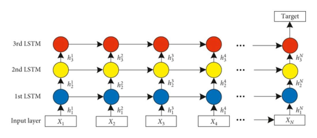
num_layers determines if the RNN is stacked (if num_layers > 1). Stacked RNNs can be thought of individual RNN modules stacked together, with the output of one module acting as input to the next RNN module. Stacked RNNs increase the complexity and expressive power of standard RNNs by adding multiple layers, allowing them to learn more sophisticated patterns in sequence data. However, this added power comes with increased computational cost and training complexity.
**This is the training and testing process:**
```python=10
# Set the model to training mode
model.train()
for data, target in train_loader:
optimizer.zero_grad()
output = model(data)
loss = loss_function(output, target)
loss.backward()
optimizer.step()
# Set the model to evaluation mode
model.eval()
with torch.no_grad():
for data, target in test_loader:
output = model(data)
# calculate metrics
```
1. model.train(): This is setting the model to training mode / indicating that the model is about to be trained. This is important because certain layers in the model behave differently during training than during testing.
2. optimizer.zero_grad(): Before the model processes a new batch of data, this line clears the old gradients. Gradients accumulated from the previous batch should not be mixed with the gradients of the current batch.
3. output = model(data): The model processes the input data (data) and produces output, which are the model's predictions for this batch. Forward propagation is done implicitly.
4. loss = loss_function(output, target): The loss function calculates the difference between the predictions (output) and the actual values (target). It quantifies how well the model is performing.
5. loss.backward(): This computes the gradient of the loss with respect to all model parameters (weights and biases) that are set to require gradients. This is where backpropagation happens.
- It's important to note that PyTorch accumulates gradients. That means each time .backward() is called, the gradients are added to the .grad attributes.
6. optimizer.step(): This updates the model parameters using the gradients computed by loss.backward(). The optimizer modifies each parameter according to the learning rate and other hyperparameters.
7. model.eval(): This should be done before evaluating or testing the model. This notifies all layers that they are in evaluation (or testing) mode, not training mode.
8. with torch.no_grad(): This tells PyTorch that gradients should not be computed in the enclosed block. This is useful because during evaluation or testing, we don't need to update the model parameters, so gradients are unnecessary.
9. output = model(data): For each batch in the test dataset, this line computes the model's predictions. This was the same line in training.
## Disadvantages
RNNs are trained using a method called backpropagation through time (BPTT). In BPTT, the error is propagated back from the output layer through each time step, updating the network’s weights to minimize the loss function. The gradients in deep neural networks are calculated using the chain rule of calculus. In RNNs, this involves multiplying the gradients across time steps or layers.
**Vanishing Gradient:** RNNs can be difficult to train because of vanishing gradients. The gradients of the loss function become increasingly small as they are propagated back through each time step or layer during training. This problem hampers the learning process, particularly in networks with long sequences or many layers. When the gradients are very small (less than 1), multiplying them over many time steps leads to an exponential decrease in their magnitude. Consequently, the gradients can become so small that they have virtually no effect in updating the weights of the neurons in earlier layers or time steps. This is known as the vanishing gradient problem. Vanishing gradients are often due to the activation functions used in the network. For example, traditional activation functions like the sigmoid or tanh function have derivatives in the range of (0, 1).
**Exploding Gradient:** This problem arises when large error gradients accumulate, leading to very large updates to the neural network model weights during the training process. The exploding gradient problem happens when the gradients of the network's weights become excessively large. This typically occurs when the derivatives of the loss function are very large, or when the gradients are multiplied together over many layers in deep networks or many time steps in RNNs, resulting in exponentially growing values. This can make the learning process unstable, leading to a situation where the model overshoots the minima of the loss function. Exploding gradients are more common in architectures with many layers or long sequences where gradients are multiplied over these many stages. Certain activation functions or initialization methods can also exacerbate the problem.
Long training time, poor performance, and bad accuracy are the key issues in gradient problems. RNNs have a short-term memory and struggle to handle long-term dependencies.
## Extensions to RNNs
There are several solutions to solve the problems related to RNNs mentioned in the previous section.
One of them is a **Long Short-Term Memory (LSTM)** which are capable of learning lengthy-time period dependencies. They remember information for a long period of time. Like standard RNNs, LSTMs process data sequentially and maintain a hidden state that is passed from one step in the sequence to the next. However, LSTMs have a more complex internal structure that allows them to store and access information over long periods effectively.
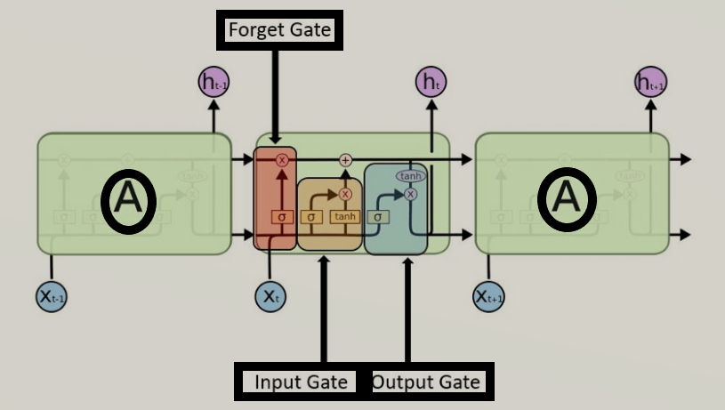
Each LSTM module may have three gates:
- Forget Gate: makes a decision on which info to be disregarded from the cell state in that unique timestamp. It looks at the previous hidden state and the current input and outputs values between 0 and 1 for each number in the cell state (1 means “keep this” and 0 means “forget this”) via sigmoid function. This determines what % of the long-term memory is remembered.
- Input Gate: updates the cell state with new information. It first decides which values to update (using a sigmoid function) and then creates a vector of new candidate values (using a tanh function) that could be added to the state. Tanh block -> Potential long-term memory. Sigmoid block -> % potential memory to remember. These determine how we should update the long-term memory.
- Output Gate: decides what the next hidden state should be. It takes the cell state and runs it through a tanh function (to push the values to be between -1 and 1) and multiplies it by the output of a sigmoid function applied to the previous hidden state and the current input, determining what part of the cell state makes it to the output. Tanh block -> potential short-term memory. Sigmoid block -> % potential memory to remember. These determine the new short-term memory (which is also the output for the entire LSTM unit).
The key to LSTMs is the cell state, the horizontal line running through the top of the diagram. It runs straight down the entire chain, with only some minor linear interactions, making it easier for information to flow along it unchanged. The cell state represents long-term memory. No weights and biases modify it directly. This allows the long-term memories to flow through a series of unrolled units without causing the gradient to explode or vanish.
The horizontal line through the bottom (hidden state) represents short-term memory. This is directly connected to weights that can modify them.
These gates and the cell state allow LSTMs to selectively remember and forget information over long sequences, making them highly effective for tasks where understanding long-term context is crucial, such as language modeling, text generation, speech recognition, and more. LSTMs mitigate the vanishing gradient problem common in traditional RNNs by using two paths (one for long-term and one for short-term), allowing them to learn from much longer sequences and capture long-term dependencies.
## Useful Links
- https://www.geeksforgeeks.org/introduction-to-recurrent-neural-network/
- https://medium.com/analytics-vidhya/understanding-rnn-implementation-in-pytorch-eefdfdb4afdb
- https://k21academy.com/datascience-blog/machine-learning/recurrent-neural-networks/
- https://youtu.be/YCzL96nL7j0