Analyzing Heat Field Deformation Sap Flow Data with the SapFlowAnalyzer: A User Guide
==============

### Abstract

This document describes the handling of the R Shiny Application SapFlowAnalyzer (SFA) to analyze heat field deformation (HFD) sap flow data. Chapters 1 and 2 provide a quick overview of the SFA, while the following chapters provide detailed information on each item of the navigation bar.

### Contents

<!-- MarkdownTOC autolink="false" style="unordered" levels="1,2" -->

- [Introduction](#Introduction)
- [Launch the SFA](#Launch-the-SFA)
- [Settings](#Settings)
- [Data](#Data)
- [K value](#K-value)
- [Sap Flow](#Sap-Flow)
- [Visualization](#Visualization)
- [Troubleshooting](#Troubleshooting)

<!-- /MarkdownTOC -->

<br>

# Introduction

The **Sap Flow Analyzer** (SFA) is a R Shiny app to process sap flow data recorded with the Heat Field Deformation (HFD) method. HFD is a thermodynamic method to measure sap flow using a continuous heating system ([Nadezhdina et al., 2006](https://doi.org/10.1093/treephys/26.10.1277); [Nadezhdina, 2018](https://doi.org/10.3832/ifor2381-011)).
With a needle-like heater a heat field is created across the stem and the heat distribution is measured with three needle-like sensors.
A needle sensor can have multiple, evenly distributed, thermocouples which record radial flow profile. Based on the ratio of temperature gradients around the heater in axial (TSym) and tangential (Tas) directions, sap flow metrics (sap flow per section, sap flow density), sap flow rate and tree water use can be estimated.
The method requires to determine a calibration value (K) for each tree and thermometer.
With the SFA, data can be cleaned or filtered, K can be determined and sap flow per section can be scaled to sap flow and total tree water use.

The following sections describe each step required to upload, filter and process data. The SFA is designed in a way that the navigation bar on the left (_Figure 1_) guides the order in which sap flow recordings are analyzed:

1. Create a project and define the measuring environment (Settings)
2. Upload data (Data)
3. Estimate K for each thermometer (K-value)
4. Calculate sap flow index (SFI), sap flow per section (SFS), sap flow density (SFD), sap flow (SF) and tree water use (TWU) (Sap flow)

The navigation bar can be collapsed by pressing the triple bar symbol (≡). The header on the top right shows the name of the current project (user determined) as well as the name of the uploaded raw data file.

<br>

# Launch the SFA

SFA can be initialized in two different ways:

1) by manually creating a local copy of the github repository,
2) by launching the app via an R wrapper function.

Both methods require the free software [R](https://cran.r-project.org/) and the R-package ‘shiny’ (version 1.5 or higher, [Chang et al., 2020](https://cran.r-project.org/package=shiny)).
To install and load the package, run the following two lines of code in an R script:

install.packages("shiny")
library("shiny")

The use of the IDE [Rstudio](https://www.rstudio.com/) is optional.

### Launching through manual start

Fork and clone (GitHub, 2022) or download the github repository https://github.com/mcwimm/SFA and navigate to the directory where the repository is stored. The main shiny app files, _server.R_ and _ui.R_, can be used to launch SFA using the ‘Run App’ button in RStudio. This method allows the user to modify the code and cooperate with the developers.

### Launching through Wrapper function

Use the ‘runGitHub’ command providing the name and the owner of the repository as well as the destination directory:

runGitHub(repo = "SFA", username = "mcwimm", destdir = NULL)

This method has the advantage, that the user always accesses the current version.
However, files are stored in a temporary folder if not previously defined by the user, and might get lost.

If the app is launched successfully it opens in a browser window, leading the user to the landing (about) page of the SFA (**<1>**), which provides some basic information about the app (**<2>**), the heat field deformation (HFD) method (**<3>**), a short guide on how to use the app (**<4>**) and output options (**<5>**).
The dash or plus in the right upper corner of each box allows to collapse each box (**<6>**).


<br>

# Settings

In the second menu item, the project settings are defined. All project settings are optional but strongly recommended for the efficient use of the SFA.

### Box `Measuring environment`

In this section of the app, the user defines wood and sensor properties.
Wood and sensor properties are crucial to calculate SFD, SF or TWU as they determine the position of each thermometer.

Wood properties (**<1>**) describe, inter alia, the stem geometry that is used to estimate thermometer positions.
If known, exact measures of sapwood and heartwood depth can be provided and used instead (**<2>**).
Sensor properties describe the spacing between needles as well as the depth of needle insertion (**<3>**).


The calculated positions can be seen at the bottom of this box.
Thermometer positions can also be defined manually.

The definition of wood and sensor properties is only required, if recordings are scaled to SFD, SF or TWU.

### Box `Project`

The user can create a project by selecting a project directory.

To create a project, press ‘Folder select’ to browse to the directory where all project files should be stored.
Choose a volume to browse in (on windows this is usually the working directory and the main drive, **<1>**).
Select a project destination folder by clicking on it's name (**<2>**).
You can also create a new subfolder by clicking **<3>**, type a name and confirm by clicking on the plus symbol **<4>**.
Finally select the folder by clicking 'select' **<5>**.


After selecting a project destination folder, press ‘Create/set project’ (**<1>**). The app automatically creates two subdirectories: ‘graphics’ and ‘csv-files’, where all the processed files are stored in.
If no project is created, all results (csv-files and graphics) are saved in the root directory of the app, which might be in the temporary data.
If the project was created successfully, the project name is shown in the upper right corner of the SFA **<3>**.
The path to the project directory is shown in **<4>**.
If no project was created, the path to the root directory is shown.


### Box `File output (optional)`

File output allow the user to define
- File format in which data files will be exported (csv, xls)- Note these files will be saved into the csv-file project folder regardless of the format selected
- the format in which figures are saved (jpeg, rdata, pdf)
- the format in which all procesed data files will be exported to (csv or excel, they will be stored in the csv-files folder of the porject)
- a title added to each saved figure, e.g. the investigated tree species
- an prefix added to the name of each saved file


### Box `Visualization (optional)`

In the Visualization box, the figure scheme ([Wickham, 2016](https://doi.org/10.1007/978-0-387-98141-3)) and colors to be used in all graphics can be defined as hex colors.


<br>

# Data

The ‘data’ menu item is divided in three subsections: upload, filter and view.

## Upload
### Box `Upload file`

To upload a csv file browse to the directory where the file is stored (**<1>**).
Select the input file type (**<2>**), the separator and the number of lines to skip (**<3>**).
If the upload is successful, the box `Preview data` shows a table with data.
To confirm the usage of the file click ‘Use data’ (**<4>**).
Afterwards, the file name is shown in the upper right corner of the SFA.
If the data is not shown correctly, open the csv-file externally and check the required column names (Table 1) and the csv-settings (i.e., comma delimited, tab delimited, etc.).


### Box `Description`

The SFA provides the option to upload csv-files of different types.
A detailed description can be found in Table 1, including the required column names.
In all cases, the data file must contain time recordings, either provided in two columns named ‘date’ and ‘time’ or in one column named ‘datetime’.
Column names are not case sensitive.

Processed data files are previous outputs of the SFA and allow to continue an analysis or produce and update figures.
In the ‘read’ mode, the existing data cannot be changed. That means, if the data file, for example, contains SFD calculated with the negative formula, this cannot be switched to the positive formula.
However, this mode allows to modify figures.
The ‘write’ mode, contrary, allows to change previously calculated results, e.g. by adjusting wood properties.

_**Table 1** Data types available in the SFA. Column names are not case sensitive._

| **Type** | **Description** | **Required columns** |
|:---------------------------------------- |:---------------------------------------------------------------------------------------------------------------------------------------------------------------------------- |:------------------------------------------------------------------------------------------------------------------------------------------------------------------------------------------------------ |
| **Raw** | Raw HFD temperature recordings, this includes temperatures recorded with the upper, side and lower sensor, respectively, at different depths. | Column names must contain the number of thermometer position _i_ and the letters U, S or L to indicate the sensor, e.g. “Temp 2 S”, “temp_1_U”. |
| **Delta** | Recordings of symmetrical and asymmetrical temperatures differences at different depths. | Columns names must contain temperature differences, dtsym and dtas at different depths _i_, e.g. “dTSym_1”, “dTas 3”. |
| **Processed read** / **Processed write** | Processed recordings of SFS, SFD, etc., preferably produced with the SFA, in long-format. That is, one column contains the results, e.g. SFD, for all thermometer positions. | Column names are fixed and case sensitive. File contains at least: dTas, dTSym, dTsa, dTsym.dTas. Further optional column names are: k, SFS, SFDsw, depth, Aring, R, Cring, SFdepth, sfM1, sfM2, sfM3. |

### Box `Preview data`

Data are shown in wide and long format (**<1, 2>**).
The latter can be downloaded as csv or excel files (**<3>**) and later used to continue the analysis using the input file types ‘Processed read’ or ‘Processed write’ from the 'input file type' drop-down menu located on the "Upload file" tab.


<br>

## Filter

### Box `Filter options`

The SFA provides different options to clean the data before processing them. This includes
- Selecting dates and times, e.g. remove the date when the sensor was installed or removed
- Selecting minimum and maximum limits for each temperature difference
- Removing outliers, separately for each temperature difference variable
- Removing rows with NA values (not available or missing values)
- Selecting individual sensor positions (e.g. only thermometers that were located in the sapwood)

To load or refresh filter options, click 'Load filter options' (**<1>**).
In case a new data set has been uploaded without refreshin the app, this button needs to be clicked, too, in order to refresh filter options (**<2>**).

By clicking ‘Apply filter’ (**<3>**), all defined changes are applied to the data set.
‘Delete filter’ resets the data set to its original extend version (**<4>**).


### Box `Figures`

In this box, the filtered data are visualized, either as violin plot, boxplot, histogram or using frequency polygons (**<1>**).
The drop-down menues 'Variable' and 'Color/ Group' determine the appearance of the image.

Filtered data can be saved as csv or excel-file (long-format) or as figure by clicking 'Save file' or 'Save figure', respectively (**<2>**).


<br>

## View

This menu item allows to create customized figures.
In the box `Settings`, the variables which are used to build the plot, e.g. axis and color vairables, are defined.
A click on ‘Render figure’ produces the graphic shown in box `Figure`.
Each figure can be saved using the 'Save figure' button.

<br>

# K value
## Description

Here a short description on how to estimate K and the type of K diagrams is provided.
A detailed discussion on the meaning of K in sap flow estimation can be found in [Nadezhdina, 2018](https://doi.org/10.3832/ifor2381-011).

## Estimation
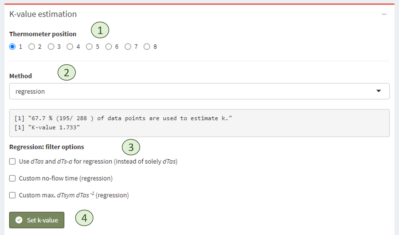
### Box `K-value estimation`

For each thermometer position, K has to be estimated.
By clicking on a radio button (**<1>**), K is estimated using the selected method (**<2>**) and optional filter options (**<3>**).
If K is estimated properly, it can be set using the ‘Set k-value’ button (**<4>**).


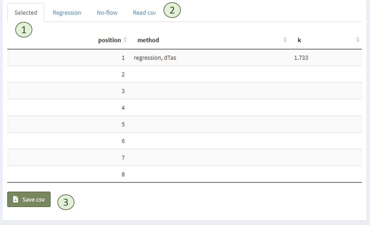
All set K values will appear in the table ‘Selected’ (**<1>**).
The other tables (**<2>**) provide estimation for all thermometer positions at once obtained with each method.
All regression options (figure above **<3>**) apply to this table, too.
If the values of this tables are sufficient, they can all be set at once by clicking ‘Use k-values’ below the table.
If K values are provided in a csv-file, the file can be uploaded in the ‘Read csv’ tab (**<2>**).
Selected K values can also be exported as data files (**<3>**).


A detailed description of K estimation using the SFA is provided in _Wimmler et al. (2023)_.

### Box `Control plots`

This box shows the typical K diagram (**<1>**) as well as two control diagrams (**<2>**) to assess the quality of the estimate.

It is possible to zoom in by defining the range of the x-axis variable by setting 'Scales' (**<3>**) to _fixed_ and defining minimum and maximum values.
If the method 'regression' is chosen to estimate K, the regression line can be forced to cross the y-axis by enabling 'Fullrange regression' in the K-diagram tab (**<4>**).

The ‘Save figures’ button (**<5>**) downloads the K-diagram as well as the two control diagrams for the selected thermometer position.


<br>

# Sap Flow
## Sap Flow Metrics

This menu item shows sap flow metrics as diurnal flow and as radial profile.
What is shown in box `Figures` needs to be defined in box `Settings`.

In the drop down menu ‘y-axis’ (box `Settings`), the user can choose which metric is shown, namely sap flow index (SFI), sap flow per section (SFS) or sap flow density (SFD).
The style options define the appearance of the figure, i.e. whether all data is presented in one figure (‘Normal’), in different panels for thermometer position or day of the year (‘Facet wrap’) or if thermometers should be grouped.
In the latter case, names of the groups and the associated thermometer positions must be provided.

The radio buttons under ‘SFS-formula’ define which formula is used to calculate SFS and hence, SFD.
Detailed information on the use of those formulas is given in [Nadezhdina and Nadezhdin, 2017](https://doi.org/10.1016/j.envexpbot.2017.04.005) and _Wimmler et al. (2022)_.
If the radio button ‘Negative’ is chosen, the negative formula is applied to each recording with SFI below a certain threshold.
The default threshold for all thermometer positions is 0°C but can be customized either with a general threshold or for each thermometer position individually.

<br>

## Tree Water Use

Sap flow rate and daily tree water can be calculated using three different upscaling methods (box `Settings`, methods are described in Wimmler et al. 2022).
Upscaling is based on sap wood depth, thus the correct definition of wood properties is essential (Settings > Measuring environment > Wood properties).

The tab ‘Diurnal pattern’ shows the total sap flow rate of a tree (or stem) over time, while tabs ‘Daily balance’ and ‘Radial profile’ show the total tree water use, which is calculated as the area under the curve of the sap flow rate (box `Figures`).

The tree water use per day is shown in the table in box `Tree water use`.

<br>

# Visualization

All produced figures can be downloaded.
The format is either jpeg, rdata or pdf and is defined under ‘Settings > File output > Figure format’.
A general figure title and appendix to figure files can be defined under ‘Figure title’ and ‘File appendix’ in the same box.
The style of figures can be customized under ‘Settings > Visualization’. Downloading figures as rdata file allows to load the figure-object to the R environment again and process the figure according to user demands.

For some figures, special settings are available.
An explanation to those options is listed below.

- **Facet wrap** Shows subsets of data presented in individual panels
- **Facet** variable that is arranged in different panels, e.g. day of the year or thermometer positions
- **No. colums** Number of columns presented in one row
- **Scales** Description by ([Wickham, Navarro and Pedersen, 2022](https://ggplot2-book.org/index.html))
- “scales = "fixed": x and y scales are fixed across all panels.
- scales = "free_x": the x scale is free, and the y scale is fixed.
- scales = "free_y": the y scale is free, and the x scale is fixed.
- scales = "free": x and y scales vary across panels.”
- **Facet grid** Similar to facet wrap. Presents data as 2d grid, defined by two variables.
- **Scales**
- **Free** x and y scale is free
- **Fixed** x and/ or y scale can be customized

<br>

# Troubleshooting

We try to provide constructive warnings or error messages.
However, we cannot catch all issues.
Below is a list with possible operating errors, their cause and a possible solution. Moreover, the output of the R console often provides a hint on what went wrong.

Please note that the App was developed and tested on a Windows system, and partially tested on mac OSX.

| **General** |
| -------- |
| &#10060; Warning in R console: Error in (...) could not find function(...)
&#10004; It is likely that not all packages were loaded. Please run the setup file ('set-up.R' located in the root directory) separately and make sure all required packages are installed. |

| **Launch the SFA** |
| -------- |
| &#10060; The SFA does not open when started via the ‘Run App’ or ‘RungGitHub’-command, or the following error message is shown: *'An error has occurred! could not find function (...)'*.
&#10004; Try to run the script ‘setup.R’ separately to install and load all required packages
&#10004; On Mac: 1) run the command `library(shiny)` (see [Launch the SFA](#Launch-the-SFA)), 2) grant access permissions to RStudio (open system preferences > Security and privacy > privacy and select "full disk access" from the left pane and click or add R Studio on the right pane). If this does not solve the problem and you are running the app through the wrapper function, then 3) you will need to also grant access to your navigation browser (i.e., Safari) as described for step 2)|

| **Data upload** |
| -------- |
| &#10060; Preview table shows error message instead of uploaded table
&#10004; Carefully check the upload settings. May open the csv file externally in a text editor and see which separator is used and how many lines need to be skipped. In some cases, the raw data file contains header sections between recordings, which can cause trouble. Delete them manually.|

| **K estimation** |
| -------- |
| &#10060; Figures do not show zero-flow axis (x=0) by default
&#10004; This seems to only occur with Mac. To change the scale of the x-axis in the diagram enable 'fixed' scales in Box `Control plots` |

| **Sap Flow Metrics** |
| -------- |
|&#10060; The SFS or SFD figures presents less thermometer positions than present in the data set
&#10004; K values were not set for all positions. Go back to K-value > Estimation and check table ‘Selected’ in the box `K-value estimation`.|

| **Sap Flow Metrics** |
| -------- |
|&#10060; Negative formula option show less SFS and SFD data than present in the data set although all K values have been set.
&#10004; More than one manual thresholds is provided but the total number of thresholds is smaller than the number of thermometers.|