---
# System prepended metadata

title: 【統計學】03 期望值、方差與共變異數
tags: [統計]

---

# 【統計學】03 期望值、方差與共變異數

[TOC]

## Part 1.　Mean / Expected Value (平均數 / 期望值)

#### 符號 : ==<span style="color:red">$E(X)$</span> 或 <span style="color:red">$\mu_X$</span>==

<br>

### 1.1　Mean of R.V. X

#### 公式
$$
E(X) = 
\left\{ 
    \begin{array}{l}
        \sum_x x\ f(x) & {\text{, if } X \text{ is discrete}} \\
        \int_x x\ f(x)dx & {\text{, if } X \text{ is continuous}}
    \end{array}
\right.
$$

> $X$ 為可替換值。

<br>

#### 其他公式
- $E\ (\ aX + b\ ) = aE(x) + b$
- $E\ [\ g(x) \pm h(x)\ ] = E[g(x)] \pm E[h(x)]$

<br>

### 1.2　Mean of Joint R. V. X and Y

#### 公式
$$
E\ [\ g(X,Y)\ ] = 
\left\{ 
    \begin{array}{l}
        \sum_x\sum_y g(x,y)\ f(x,y) & {\text{, if } X,Y \text{ are discrete}} \\
        \int_x\int_y \ g(x,y)\ f(x,y)dxdy & {\text{, if } X,Y \text{ are continuous}}
    \end{array}
\right.
$$

> $g(X,Y)$ 為可替換值。

#### Note : ==$X \text{ and } Y$ <span style="color:red">$\text{ independent }$</span> $\implies$ <span style="color:red">$f(X,Y) = f(X) \cdot f(Y)$</span>==

<br>

#### 其他公式
- $E(aX \pm bY) = aE(X) \pm bE(Y)$
- $E[g(X,Y) \pm h(X,Y)] = E[g(X,Y)] \pm E[h(X,Y)]$

<br>

---

## Part 2.　Variance (方差/變異數/離散度)
用於表示一組數值資料中的各數值相對於該組數值資料之平均數的分散程度。

#### 符號 : ==<span style="color:red">$Var(X)$</span> 或 <span style="color:red">$\sigma_X ^ 2$</span>==

**$\sigma_X ^ 2$ 開根號後 $\to$ 即為標準差 (standard deviation, 符號 $\sigma$ )，也稱均方差 (mean square error) $\to$ same measuring unit of $X$**

<br>


#### 公式
$$
Var(X) = E\ [(X - \mu_{X})^2] = 
\left\{ 
    \begin{array}{l}
        \sum_x (x - \mu_{X})^2\ f(x) & {\text{, if } X \text{ is discrete}} \\
        \int_x \ (x - \mu_{X})^2\ f(x)dx & {\text{, if } X \text{ is continuous}}
    \end{array}
\right.
$$

$\implies$ ==$Var(X) = E(X^2) - \mu_X^2 = E(X^2) - [E(X)]^2$==
> $X$ 為可替換值。

<br>

#### 其他公式
- $Var(aX + b) = a^2Var(X)$

<br>


---

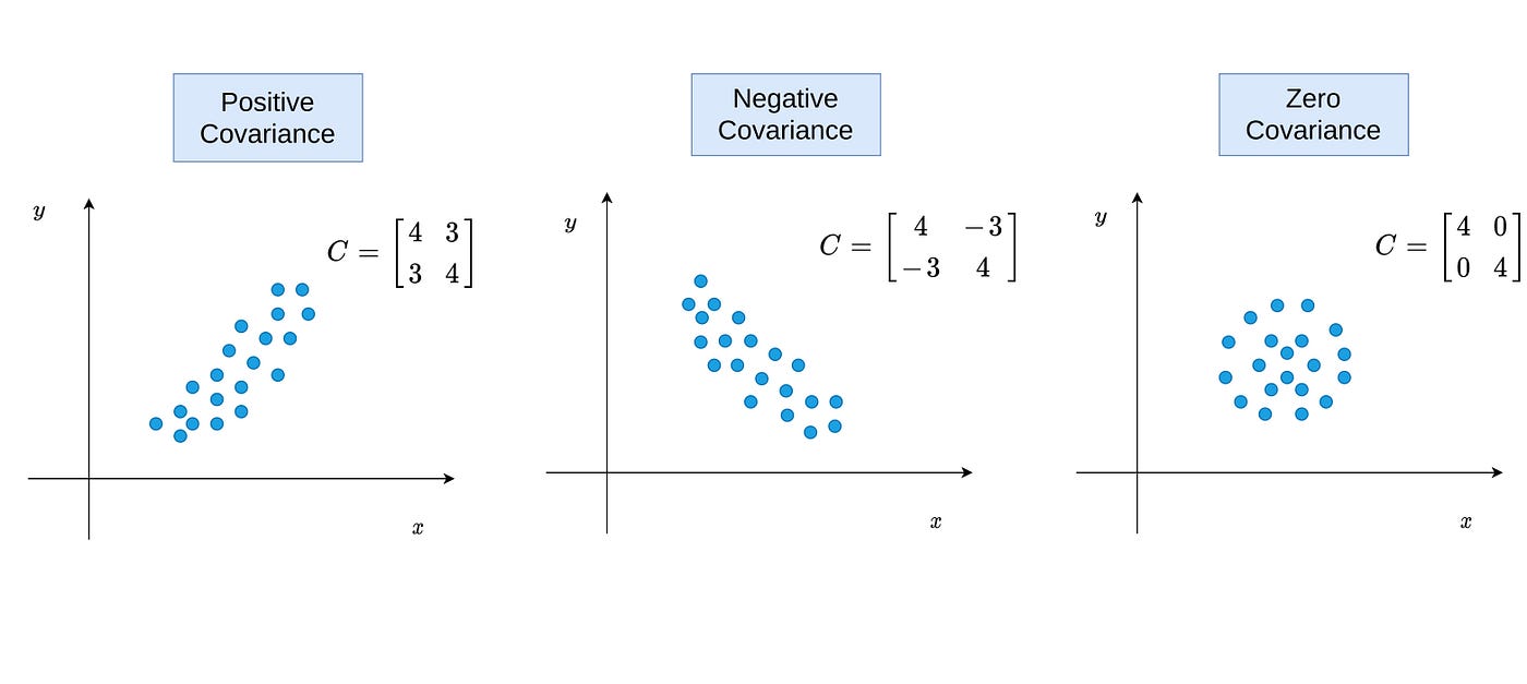
## Part 3.　Covariance (共變異數)
共變異數描述 $X$ 與 $Y$ 之間的<span style="color:red">線性(linear)關係</span> $\implies$ <span style="color:blue">無法顯示非線性(non-linear)關係，以及關係的強度(strength)</span>
<br>

#### 公式
$$
Cov(X,Y) = E[(X - \mu_{X})(Y - \mu_{Y})] = 
\left\{ 
    \begin{array}{l}
        \sum_x\sum_y (x - \mu_{X})(y - \mu_{Y})\ f(x,y) & {\text{, if } X,Y \text{ are discrete}} \\
        \int_x\int_y \ (x - \mu_{X})(y - \mu_{Y})\ f(x,y)dxdy & {\text{, if } X,Y \text{ are continuous}}
    \end{array}
\right.
$$
$\implies$ ==$Cov(X,Y) = E(XY) - \mu_X\mu_Y$==<br>
$\implies Cov(X,X) = E(X^2) - \mu_X^2 = Var(X)$
<br>

### 3.1　Convariance Matrix
- $Cov(X,Y) = Cov(Y,X)$
- $Cov(X+Y, W+Z) = Cov(X,W) + Cov(X,Z) + Cov(Y,W) + Cov(Y,Z)$
- $Cov(aX,bY) = abCov(X,Y)$
- $Var(\bar{X}) = Cov(\bar{X}, \bar{X}) = Cov(\frac{1}{n}X_1 + \cdots + \frac{1}{n}X_n,\  \frac{1}{n}X_1 + \cdots + \frac{1}{n}X_n)$
   <br> &nbsp;&nbsp;&nbsp;&nbsp;&nbsp;&nbsp;&nbsp;&nbsp;&nbsp;&nbsp;&nbsp;&nbsp;&nbsp;&nbsp;$=$ ==$\frac{1}{n^2} \sum_{i=1}^nVar(X_i) + 2 \cdot \frac{1}{n^2}\sum_{i<j}Cov(X_i, X_j)$==

<br>

&nbsp;&nbsp;&nbsp;&nbsp;&nbsp;&nbsp;&nbsp;&nbsp;&nbsp;&nbsp;&nbsp;&nbsp;&nbsp;&nbsp;&nbsp;&nbsp;&nbsp;&nbsp;&nbsp;&nbsp;&nbsp;&nbsp;&nbsp;&nbsp;&nbsp;&nbsp;&nbsp;&nbsp;&nbsp;&nbsp;&nbsp;&nbsp;&nbsp; <img  style="width:250px" src='https://www.researchgate.net/publication/237014579/figure/fig1/AS:213963448033280@1428024269392/Variance-covariance-matrix-depicting-homogeneity-of-variance-and-compound-symmetry.png'>
<br>
>  如果 $X_1, \dots, X_n$ 是獨立 (independent) 且具有相同分佈 (identically distributed) (i.i.d.)，則 $E(\bar{X}) = E(X_i)$ 以及 $Var(\bar{X}) = \frac{Var(X_i)}{n}$

<br>

### 3.2　共變異數特性 (關係)
- $Cov(X,Y)$ 反映 $X$ 與 $Y$ "move together" 的動向
    - <span style="color:blue">$Cov(X, Y) > 0 \to$ positively correlated</span>
    - <span style="color:blue">$Cov(X, Y) < 0 \to$ negatively correlated</span>
    - <span style="color:red">$X \text{ and } Y \text{ are independent (uncorrelated) } \to Cov(X, Y) = 0 \text{ and } E(XY) = E(X) \cdot E(Y)$</span>
- <span style="color:red">$Cov(X,Y) = 0 \ne \text{ independent }$</span>，因為 Covariance 只顯示線性關係，不能說明是否存在非線性關係。 
    <img src='https://miro.medium.com/v2/resize:fit:1400/1*S0eywPhsOOLcvPIOrhz6_A.jpeg'>
- ==$Var(aX \pm bY) = a^2Var(X) \pm 2abCov(X,Y) + b^2Var(Y)$==
- 變異數不會是負的，如果 $X$ 和 $Y$ 是獨立的 $\implies Var(X - Y) = Var(X) + Var(Y)$ 
- 如果 $X_1, X_2, \dots, X_n$ 是獨立的 $\implies Var(\sum^n_{i=1}a_iX_i) = \sum^n_{i=1}a^2_iVar(X_i)$

<br>
    
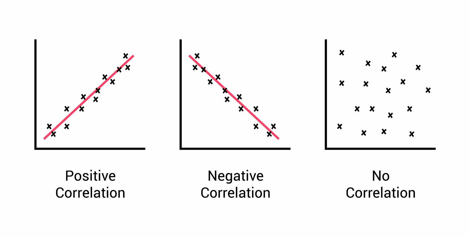
### 3.3　相關係數 (Correlation coefficient)
$Cov(X,Y)$ 並不能顯示線性關係的「強度(strength)」，因為 $Cov(X,Y)$ 會**受使用單位影響**，故需使用 <span style="color:blue">相關係數(correlation coefficient)</span>。
    
#### 公式
$\rho_{XY} = \dfrac{Cov(X,Y)}{\sigma_X\sigma_Y} = Cov(\dfrac{X}{\sigma_X}, \dfrac{Y}{\sigma_Y})$
> $\sigma_X$ 和 $\sigma_Y$ 是 <span style="color:red">scale-free</span>
    
#### 值域
<span style="color:green">(負相關) $-1 \le \rho_{XY} \le 1$ (正相關)</span>
    
<img style="width:500px" src='https://www.simplypsychology.org/wp-content/uploads/correlation.jpg'><br>
    

---
    
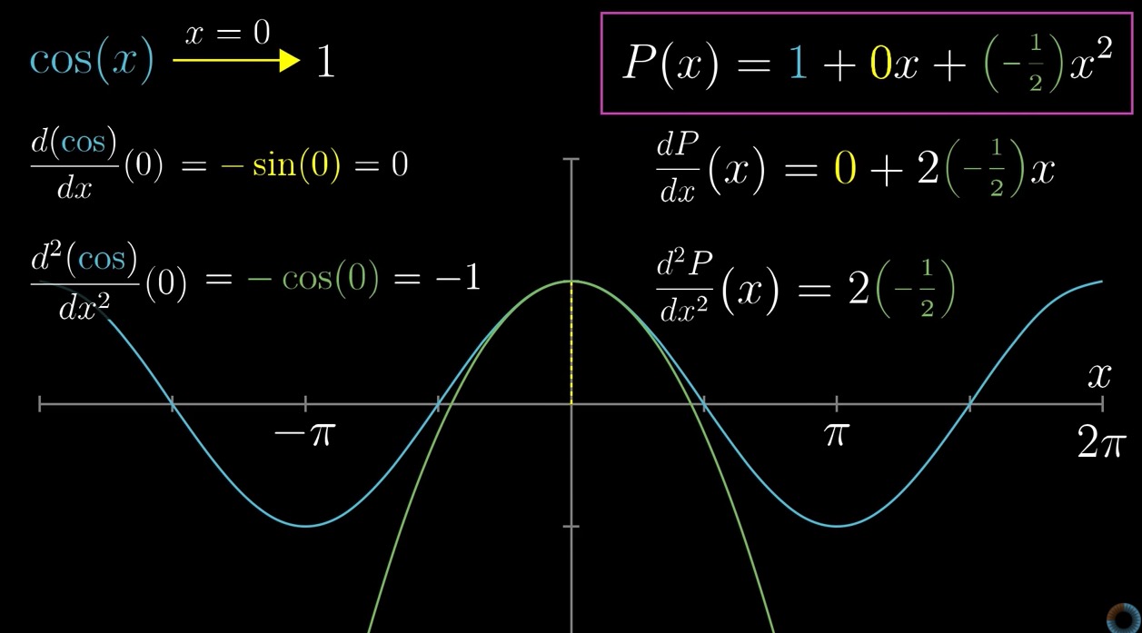
## Part 4. Taylor series approximation

<img style="width:500px" src='https://publish-01.obsidian.md/access/fc5a2dd092cb06eefdd04ff307334d7a/_attachments/approximation%20of%20cosine%20using%20derivatives.jpg'><br>
    
<img style="width:500px" src='https://publish-01.obsidian.md/access/fc5a2dd092cb06eefdd04ff307334d7a/_attachments/geometric%20interpretation%20of%20taylor.jpg'><br>

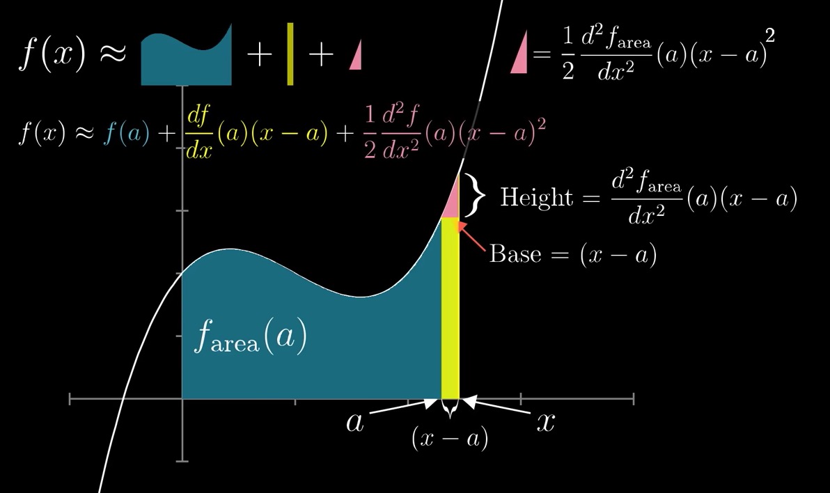
在上圖中，$Height = (Slope) \cdot (x-a)$，斜率 $= \frac{\Delta{y}}{\Delta{x}}$
    
<br>
    
---
    
## Part 5. 標準差 (Standard deviation)
隨機變數與平均值的「平均距離」，作為標準單位來衡量 <span style="color:blue">"deviations" $X - \mu$</span>