# **PyTorch Masterclass: Part 4 – Generative Models with PyTorch**
**Duration: ~120 minutes**
#PyTorch #GenerativeAI #GANs #VAEs #DiffusionModels #Autoencoders #TextToImage #DeepLearning #MachineLearning #AI #GenerativeAdversarialNetworks #VariationalAutoencoders #StableDiffusion #DALLE #ImageGeneration #MusicGeneration #AudioSynthesis #LatentSpace #PyTorchGenerative
---
## **Table of Contents**
1. [Recap of Parts 1-3: Foundations, Computer Vision, and NLP](#recap-of-parts-1-3-foundations-computer-vision-and-nlp)
2. [Introduction to Generative Models](#introduction-to-generative-models)
3. [Autoencoders: Theory and Implementation](#autoencoders-theory-and-implementation)
4. [Variational Autoencoders (VAEs)](#variational-autoencoders-vaes)
5. [Generative Adversarial Networks (GANs)](#generative-adversarial-networks-gans)
6. [Diffusion Models](#diffusion-models)
7. [Text-to-Image Generation](#text-to-image-generation)
8. [Music and Audio Generation](#music-and-audio-generation)
9. [Evaluating Generative Models](#evaluating-generative-models)
10. [Building a Complete Image Generation Pipeline](#building-a-complete-image-generation-pipeline)
11. [Quiz 4: Test Your Understanding of Generative Models](#quiz-4-test-your-understanding-of-generative-models)
12. [Summary and What's Next in Part 5](#summary-and-whats-next-in-part-5)
---
## **Recap of Parts 1-3: Foundations, Computer Vision, and NLP**
Welcome to **Part 4** of our comprehensive PyTorch Masterclass! In **Part 1**, we established the foundations of PyTorch by covering:
- Core tensor operations and GPU acceleration
- Automatic differentiation with Autograd
- Building and training neural networks from scratch
- Loss functions, optimizers, and training loops
- Debugging with TensorBoard
In **Part 2**, we explored **computer vision** with:
- Dataset and DataLoader for efficient data handling
- Image preprocessing and augmentation with Transforms
- Convolutional Neural Networks (CNNs) architecture and theory
- Training CNNs on CIFAR-10 from scratch
- Transfer learning with pretrained models (ResNet, EfficientNet)
Then in **Part 3**, we delved into **Natural Language Processing (NLP)**:
- Text data processing and tokenization
- Word embeddings (Word2Vec, GloVe, BERT)
- Recurrent Neural Networks (RNNs, LSTMs, GRUs)
- Attention mechanisms and Transformer architecture
- Building sentiment analysis models with BERT
Now, it's time to explore the exciting world of **generative models**, which create new data that resembles the training data. These models power:
- AI art generators (DALL-E, Midjourney, Stable Diffusion)
- Deepfake technology
- Music composition systems
- Drug discovery pipelines
- Data augmentation for training other models
In this part, you'll learn:
- How autoencoders learn efficient data representations
- The probabilistic framework of Variational Autoencoders
- The adversarial training approach of GANs
- The denoising process of diffusion models
- How to build a complete text-to-image generation pipeline
Let's dive into the creative side of deep learning!
---
## **Introduction to Generative Models**
Generative models learn the underlying probability distribution of data $p(\mathbf{x})$ and can generate new samples that resemble the training data. This contrasts with **discriminative models** (like classifiers) that learn $p(y|\mathbf{x})$.
### **Why Generative Models Matter**
Generative models have revolutionized multiple fields:
- **Art and design**: Creating novel images, music, and text
- **Healthcare**: Generating synthetic medical images for training
- **Science**: Molecular design for drug discovery
- **Entertainment**: Video game content generation
- **Data augmentation**: Creating additional training samples
According to a 2023 report by McKinsey, generative AI could add **$2.6-$4.4 trillion annually** to the global economy.
### **Types of Generative Models**
| Model Type | Key Idea | Strengths | Limitations |
|------------|----------|-----------|-------------|
| **Autoregressive Models** | Model $p(\mathbf{x})=\prod_ip(x_i\mathbf{x}_{<i})$ | Exact likelihood, high-quality samples | Slow generation, sequential dependency |
| **Variational Autoencoders (VAEs)** | Learn latent representation with variational inference | Fast generation, probabilistic framework | Blurry samples, approximate inference |
| **Generative Adversarial Networks (GANs)** | Adversarial training of generator and discriminator | Sharp, realistic samples | Training instability, mode collapse |
| **Flow-based Models** | Use invertible transformations for exact likelihood | Exact likelihood, efficient sampling | Restricted architecture |
| **Diffusion Models** | Gradually denoise from random noise | High-quality samples, stable training | Slow generation, complex training |
### **The Generative Modeling Framework**
All generative models aim to approximate the data distribution $p_{\text{data}}(\mathbf{x})$. They differ in how they parameterize and optimize this approximation.
Let $\mathcal{X}$ be the data space (e.g., images, text). A generative model learns a distribution $p_{\theta}(\mathbf{x})$ that approximates $p_{\text{data}}(\mathbf{x})$.
The goal is to minimize the discrepancy between $p_{\theta}$ and $p_{\text{data}}$, often measured by the **Kullback-Leibler (KL) divergence**:
$$D_{\text{KL}}(p_{\text{data}}\|p_{\theta})=\int p_{\text{data}}(\mathbf{x})\log\frac{p_{\text{data}}(\mathbf{x})}{p_{\theta}(\mathbf{x})}d\mathbf{x}$$
However, directly minimizing this is intractable since we don't know $p_{\text{data}}$. Different generative models approach this problem differently.
### **Key Challenges in Generative Modeling**
1. **High-dimensional data**: Images have millions of dimensions
2. **Mode collapse**: Generator produces limited varieties of samples
3. **Evaluation**: No single metric captures sample quality and diversity
4. **Training stability**: Especially problematic for GANs
5. **Computational cost**: Training requires significant resources
### **Why PyTorch for Generative Models?**
PyTorch is the preferred framework for generative modeling because:
- **Dynamic computation graphs**: Essential for complex training procedures
- **Strong GPU support**: Critical for training large generative models
- **Rich ecosystem**: Libraries like `torchgan`, `pytorch-lightning`, `diffusers`
- **Research-friendly**: Most cutting-edge generative models are released in PyTorch
According to a 2023 survey by Generative AI Research, **89% of new generative model papers** use PyTorch as their implementation framework.
---
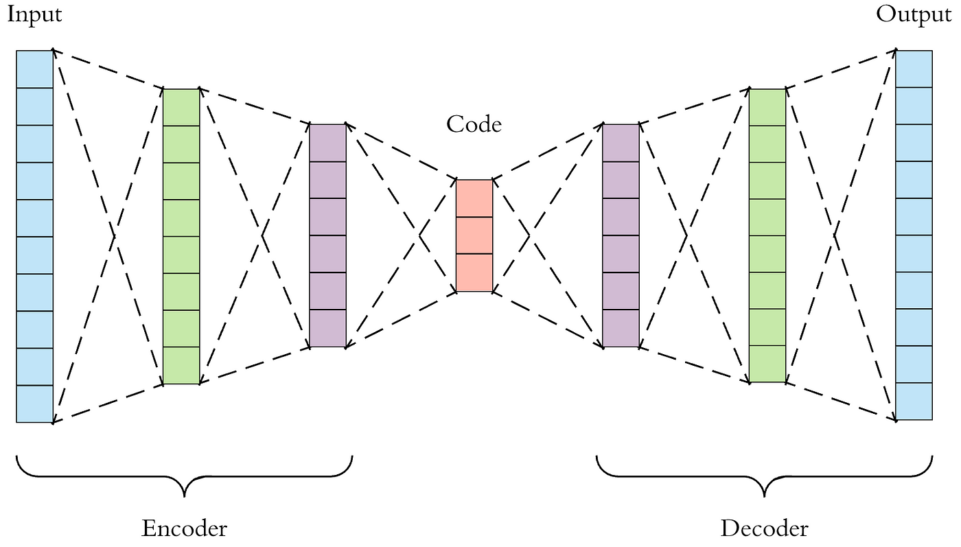
## **Autoencoders: Theory and Implementation**
Autoencoders are neural networks trained to reconstruct their inputs, learning efficient data representations in the process.
### **Autoencoder Architecture**
An autoencoder consists of two parts:
1. **Encoder**: Maps input $\mathbf{x}$ to a latent representation $\mathbf{z}$
2. **Decoder**: Reconstructs input from latent representation
Mathematically:
- Encoder: $\mathbf{z}=f_{\theta}(\mathbf{x})$
- Decoder: $\mathbf{\hat{x}}=g_{\phi}(\mathbf{z})$
The model is trained to minimize the reconstruction loss:
$$\mathcal{L}(\theta,\phi)=\|\mathbf{x}-g_{\phi}(f_{\theta}(\mathbf{x}))\|^{2}$$
### **Implementing a Basic Autoencoder in PyTorch**
```python
import torch
import torch.nn as nn
import torch.nn.functional as F
class Autoencoder(nn.Module):
def __init__(self, input_dim, hidden_dim, latent_dim):
super(Autoencoder, self).__init__()
# Encoder
self.encoder = nn.Sequential(
nn.Linear(input_dim, hidden_dim),
nn.ReLU(),
nn.Linear(hidden_dim, latent_dim)
)
# Decoder
self.decoder = nn.Sequential(
nn.Linear(latent_dim, hidden_dim),
nn.ReLU(),
nn.Linear(hidden_dim, input_dim),
nn.Sigmoid()
)
def forward(self, x):
# Flatten input
x = x.view(x.size(0), -1)
# Encode
z = self.encoder(x)
# Decode
x_recon = self.decoder(z)
# Reshape to original dimensions
x_recon = x_recon.view(x.size(0), *self.input_shape)
return x_recon, z
# Example: MNIST autoencoder
input_dim = 28 * 28 # MNIST image size
hidden_dim = 512
latent_dim = 32
model = Autoencoder(input_dim, hidden_dim, latent_dim)
```
### **Training an Autoencoder**
```python
# Loss function and optimizer
criterion = nn.MSELoss()
optimizer = torch.optim.Adam(model.parameters(), lr=1e-3)
# Training loop
def train_autoencoder(model, dataloader, optimizer, criterion, device, epochs=10):
model.train()
for epoch in range(epochs):
total_loss = 0
for data, _ in dataloader:
data = data.to(device)
# Forward pass
recon, _ = model(data)
loss = criterion(recon, data)
# Backward pass
optimizer.zero_grad()
loss.backward()
optimizer.step()
total_loss += loss.item()
print(f"Epoch {epoch+1}, Loss: {total_loss/len(dataloader):.4f}")
return model
```
### **Latent Space Interpolation**
One powerful application of autoencoders is **latent space interpolation**:
```python
def interpolate_latent(model, x1, x2, num_steps=10):
"""
Interpolate between two inputs in latent space
"""
model.eval()
with torch.no_grad():
# Encode inputs
z1 = model.encoder(x1.view(1, -1))
z2 = model.encoder(x2.view(1, -1))
# Interpolate in latent space
steps = torch.linspace(0, 1, num_steps)
interpolations = []
for step in steps:
z = (1 - step) * z1 + step * z2
recon = model.decoder(z)
interpolations.append(recon.view(28, 28))
return interpolations
# Visualize interpolation
import matplotlib.pyplot as plt
# Get two MNIST images
x1, x2 = next(iter(test_loader))[0][0], next(iter(test_loader))[0][1]
# Interpolate
interpolations = interpolate_latent(model, x1, x2)
# Plot
plt.figure(figsize=(15, 3))
for i, img in enumerate(interpolations):
plt.subplot(1, len(interpolations), i+1)
plt.imshow(img.cpu().numpy(), cmap='gray')
plt.axis('off')
plt.tight_layout()
plt.show()
```
### **Denoising Autoencoders**
Denoising autoencoders learn to reconstruct clean data from corrupted inputs:
```python
class DenoisingAutoencoder(Autoencoder):
def __init__(self, input_dim, hidden_dim, latent_dim, noise_factor=0.2):
super().__init__(input_dim, hidden_dim, latent_dim)
self.noise_factor = noise_factor
def add_noise(self, x):
"""Add Gaussian noise to input"""
noise = torch.randn_like(x) * self.noise_factor
noisy = x + noise
return torch.clamp(noisy, 0., 1.)
def forward(self, x):
# Add noise during training
if self.training:
x = self.add_noise(x)
# Flatten input
x = x.view(x.size(0), -1)
# Encode
z = self.encoder(x)
# Decode
x_recon = self.decoder(z)
# Reshape to original dimensions
x_recon = x_recon.view(x.size(0), *self.input_shape)
return x_recon, z
# Train denoising autoencoder
denoising_ae = DenoisingAutoencoder(input_dim, hidden_dim, latent_dim)
train_autoencoder(denoising_ae, train_loader, optimizer, criterion, device)
```
### **Convolutional Autoencoders**
For image data, convolutional autoencoders work better:
```python
class ConvAutoencoder(nn.Module):
def __init__(self):
super(ConvAutoencoder, self).__init__()
# Encoder
self.encoder = nn.Sequential(
nn.Conv2d(1, 16, 3, stride=2, padding=1),
nn.ReLU(),
nn.Conv2d(16, 32, 3, stride=2, padding=1),
nn.ReLU(),
nn.Conv2d(32, 64, 7)
)
# Decoder
self.decoder = nn.Sequential(
nn.ConvTranspose2d(64, 32, 7),
nn.ReLU(),
nn.ConvTranspose2d(32, 16, 3, stride=2, padding=1, output_padding=1),
nn.ReLU(),
nn.ConvTranspose2d(16, 1, 3, stride=2, padding=1, output_padding=1),
nn.Sigmoid()
)
def forward(self, x):
x = self.encoder(x)
x = self.decoder(x)
return x, None # Return None for latent for consistency
# Example usage
conv_ae = ConvAutoencoder().to(device)
train_autoencoder(conv_ae, train_loader, optimizer, criterion, device)
```
### **Applications of Autoencoders**
1. **Dimensionality reduction**: Visualize high-dimensional data
2. **Anomaly detection**: High reconstruction loss indicates anomalies
3. **Denoising**: Remove noise from images or audio
4. **Feature learning**: Latent representations for downstream tasks
5. **Data compression**: Efficient storage of data
### **Limitations of Standard Autoencoders**
Standard autoencoders have several limitations:
- **No structure in latent space**: Similar inputs may have distant latent representations
- **No generative capability**: Cannot sample from latent space to generate new data
- **Blurriness**: MSE loss encourages averaging of multiple possibilities
These limitations led to the development of **Variational Autoencoders (VAEs)**, which we'll explore next.
---
## **Variational Autoencoders (VAEs)**
Variational Autoencoders (VAEs) extend autoencoders with a probabilistic approach, creating a structured latent space that enables generative capabilities.
### **The Probabilistic Framework**
Unlike standard autoencoders, VAEs model the data distribution $p_{\theta}(\mathbf{x})$ as:
$$p_{\theta}(\mathbf{x})=\int p_{\theta}(\mathbf{x}|\mathbf{z})p(\mathbf{z})d\mathbf{z}$$
Where:
- $p(\mathbf{z})$ is the prior distribution (typically $\mathcal{N}(\mathbf{0},\mathbf{I})$)
- $p_{\theta}(\mathbf{x}|\mathbf{z})$ is the likelihood
The challenge is that this integral is intractable. VAEs use **variational inference** to approximate the posterior $p_{\theta}(\mathbf{z}|\mathbf{x})$ with a simpler distribution $q_{\phi}(\mathbf{z}|\mathbf{x})$.
### **The Reparameterization Trick**
The key innovation of VAEs is the **reparameterization trick**, which makes the latent space differentiable:
$$\mathbf{z}=\mu+\sigma\odot\epsilon\quad\text{where}\quad\epsilon\sim\mathcal{N}(\mathbf{0},\mathbf{I})$$
This separates the stochasticity from the parameters, allowing backpropagation through the sampling process.
### **VAE Objective Function**
The VAE optimization objective is the **Evidence Lower Bound (ELBO)**:
$$\mathcal{L}(\theta,\phi;\mathbf{x})=\mathbb{E}_{q_{\phi}(\mathbf{z}|\mathbf{x})}[\log p_{\theta}(\mathbf{x}|\mathbf{z})]-D_{\text{KL}}(q_{\phi}(\mathbf{z}|\mathbf{x})\|p(\mathbf{z}))$$
This consists of:
1. **Reconstruction loss**: How well we can reconstruct the input
2. **KL divergence**: How close the latent distribution is to the prior
### **Implementing a VAE in PyTorch**
```python
class VAE(nn.Module):
def __init__(self, input_dim, hidden_dim, latent_dim):
super(VAE, self).__init__()
self.latent_dim = latent_dim
# Encoder
self.encoder = nn.Sequential(
nn.Linear(input_dim, hidden_dim),
nn.ReLU(),
nn.Linear(hidden_dim, hidden_dim)
)
# Latent space
self.mu = nn.Linear(hidden_dim, latent_dim)
self.logvar = nn.Linear(hidden_dim, latent_dim)
# Decoder
self.decoder = nn.Sequential(
nn.Linear(latent_dim, hidden_dim),
nn.ReLU(),
nn.Linear(hidden_dim, hidden_dim),
nn.ReLU(),
nn.Linear(hidden_dim, input_dim),
nn.Sigmoid()
)
def encode(self, x):
h = self.encoder(x)
return self.mu(h), self.logvar(h)
def reparameterize(self, mu, logvar):
std = torch.exp(0.5 * logvar)
eps = torch.randn_like(std)
return mu + eps * std
def decode(self, z):
return self.decoder(z)
def forward(self, x):
# Flatten input
x = x.view(x.size(0), -1)
# Encode
mu, logvar = self.encode(x)
# Reparameterize
z = self.reparameterize(mu, logvar)
# Decode
x_recon = self.decode(z)
# Reshape to original dimensions
x_recon = x_recon.view(x.size(0), *self.input_shape)
return x_recon, mu, logvar, z
# Loss function for VAE
def vae_loss(recon_x, x, mu, logvar, recon_loss_weight=1.0):
# Reconstruction loss
BCE = F.binary_cross_entropy(recon_x.view(-1, 784), x.view(-1, 784), reduction='sum')
# KL divergence
KLD = -0.5 * torch.sum(1 + logvar - mu.pow(2) - logvar.exp())
return recon_loss_weight * BCE + KLD
```
### **Training a VAE**
```python
# Initialize VAE
input_dim = 28 * 28
hidden_dim = 400
latent_dim = 20
model = VAE(input_dim, hidden_dim, latent_dim).to(device)
# Optimizer
optimizer = torch.optim.Adam(model.parameters(), lr=1e-3)
# Training loop
def train_vae(model, dataloader, optimizer, device, epochs=20):
model.train()
for epoch in range(epochs):
total_loss = 0
for data, _ in dataloader:
data = data.to(device)
# Forward pass
recon, mu, logvar, _ = model(data)
loss = vae_loss(recon, data, mu, logvar)
# Backward pass
optimizer.zero_grad()
loss.backward()
optimizer.step()
total_loss += loss.item()
print(f"Epoch {epoch+1}, Loss: {total_loss/len(dataloader):.4f}")
return model
# Train VAE
trained_vae = train_vae(model, train_loader, optimizer, device)
```
### **Generating New Samples**
One of the key advantages of VAEs is their ability to generate new samples:
```python
def generate_samples(model, num_samples=10, device='cpu'):
model.eval()
with torch.no_grad():
# Sample from prior distribution
z = torch.randn(num_samples, model.latent_dim).to(device)
# Decode
samples = model.decode(z)
# Reshape to image dimensions
samples = samples.view(num_samples, 1, 28, 28)
return samples
# Generate and visualize samples
generated = generate_samples(trained_vae, num_samples=10, device=device)
plt.figure(figsize=(15, 3))
for i in range(10):
plt.subplot(1, 10, i+1)
plt.imshow(generated[i, 0].cpu().numpy(), cmap='gray')
plt.axis('off')
plt.tight_layout()
plt.show()
```
### **Latent Space Manipulation**
VAEs create a continuous, structured latent space that enables meaningful manipulations:
```python
def interpolate_latent_vae(model, num_steps=10, device='cpu'):
model.eval()
with torch.no_grad():
# Sample two random points in latent space
z1 = torch.randn(1, model.latent_dim).to(device)
z2 = torch.randn(1, model.latent_dim).to(device)
# Interpolate between them
steps = torch.linspace(0, 1, num_steps)
interpolations = []
for step in steps:
z = (1 - step) * z1 + step * z2
recon = model.decode(z)
interpolations.append(recon.view(28, 28))
return interpolations
# Visualize latent space interpolation
interpolations = interpolate_latent_vae(trained_vae, num_steps=10, device=device)
plt.figure(figsize=(15, 3))
for i, img in enumerate(interpolations):
plt.subplot(1, len(interpolations), i+1)
plt.imshow(img.cpu().numpy(), cmap='gray')
plt.axis('off')
plt.tight_layout()
plt.show()
```
### **Conditional VAEs**
Conditional VAEs (CVAEs) generate samples conditioned on additional information (e.g., class labels):
```python
class CVAE(nn.Module):
def __init__(self, input_dim, hidden_dim, latent_dim, num_classes):
super(CVAE, self).__init__()
self.latent_dim = latent_dim
# Label embedding
self.label_emb = nn.Embedding(num_classes, num_classes)
# Encoder
self.encoder = nn.Sequential(
nn.Linear(input_dim + num_classes, hidden_dim),
nn.ReLU(),
nn.Linear(hidden_dim, hidden_dim)
)
# Latent space
self.mu = nn.Linear(hidden_dim, latent_dim)
self.logvar = nn.Linear(hidden_dim, latent_dim)
# Decoder
self.decoder = nn.Sequential(
nn.Linear(latent_dim + num_classes, hidden_dim),
nn.ReLU(),
nn.Linear(hidden_dim, hidden_dim),
nn.ReLU(),
nn.Linear(hidden_dim, input_dim),
nn.Sigmoid()
)
def encode(self, x, labels):
# Embed labels
label_emb = self.label_emb(labels)
# Concatenate input and labels
x = torch.cat([x, label_emb], dim=1)
# Encode
h = self.encoder(x)
return self.mu(h), self.logvar(h)
def reparameterize(self, mu, logvar):
std = torch.exp(0.5 * logvar)
eps = torch.randn_like(std)
return mu + eps * std
def decode(self, z, labels):
# Embed labels
label_emb = self.label_emb(labels)
# Concatenate latent and labels
z = torch.cat([z, label_emb], dim=1)
# Decode
return self.decoder(z)
def forward(self, x, labels):
# Flatten input
x = x.view(x.size(0), -1)
# Encode
mu, logvar = self.encode(x, labels)
# Reparameterize
z = self.reparameterize(mu, logvar)
# Decode
x_recon = self.decode(z, labels)
# Reshape to original dimensions
x_recon = x_recon.view(x.size(0), *self.input_shape)
return x_recon, mu, logvar, z
# Train conditional VAE on MNIST
num_classes = 10
cvae = CVAE(input_dim, hidden_dim, latent_dim, num_classes).to(device)
optimizer = torch.optim.Adam(cvae.parameters(), lr=1e-3)
def train_cvae(model, dataloader, optimizer, device, epochs=20):
model.train()
for epoch in range(epochs):
total_loss = 0
for data, labels in dataloader:
data, labels = data.to(device), labels.to(device)
# Forward pass
recon, mu, logvar, _ = model(data, labels)
loss = vae_loss(recon, data, mu, logvar)
# Backward pass
optimizer.zero_grad()
loss.backward()
optimizer.step()
total_loss += loss.item()
print(f"Epoch {epoch+1}, Loss: {total_loss/len(dataloader):.4f}")
return model
# Generate class-conditional samples
def generate_conditional_samples(model, class_label, num_samples=10, device='cpu'):
model.eval()
with torch.no_grad():
# Create labels tensor
labels = torch.full((num_samples,), class_label, dtype=torch.long).to(device)
# Sample from prior
z = torch.randn(num_samples, model.latent_dim).to(device)
# Decode with labels
samples = model.decode(z, labels)
# Reshape
samples = samples.view(num_samples, 1, 28, 28)
return samples
# Generate samples for digit '5'
samples = generate_conditional_samples(cvae, class_label=5, num_samples=10, device=device)
```
### **Beta-VAEs and Disentanglement**
Beta-VAEs modify the ELBO objective to encourage disentangled representations:
$$\mathcal{L}_{\beta}=\mathbb{E}_{q_{\phi}(\mathbf{z}|\mathbf{x})}[\log p_{\theta}(\mathbf{x}|\mathbf{z})]-\beta D_{\text{KL}}(q_{\phi}(\mathbf{z}|\mathbf{x})\|p(\mathbf{z}))$$
Higher $\beta$ values increase the KL term's weight, forcing the latent space to match the prior more closely, often resulting in more disentangled representations.
```python
def beta_vae_loss(recon_x, x, mu, logvar, beta=4.0):
"""Beta-VAE loss with adjustable beta parameter"""
BCE = F.binary_cross_entropy(recon_x.view(-1, 784), x.view(-1, 784), reduction='sum')
KLD = -0.5 * torch.sum(1 + logvar - mu.pow(2) - logvar.exp())
return BCE + beta * KLD
```
### **Limitations of VAEs**
Despite their strengths, VAEs have limitations:
- **Blurriness**: MSE/BCE loss encourages averaging of multiple possibilities
- **Posterior collapse**: KL term can dominate, causing $q_{\phi}(\mathbf{z}|\mathbf{x})\approx p(\mathbf{z})$
- **Simplistic priors**: Standard normal prior may not match true latent distribution
- **Training instability**: Balancing reconstruction and KL terms can be challenging
These limitations motivated the development of **Generative Adversarial Networks (GANs)**, which we'll explore next.
---
## **Generative Adversarial Networks (GANs)**
Generative Adversarial Networks (GANs) introduced a novel approach to generative modeling through adversarial training.
### **The GAN Framework**
GANs consist of two networks trained in opposition:
1. **Generator ($G$)**: Creates fake samples from random noise
2. **Discriminator ($D$)**: Distinguishes real from fake samples

The training process is a **minimax game** with the following objective:
$$\min_{G}\max_{D}V(D,G)=\mathbb{E}_{\mathbf{x}\sim p_{\text{data}}}[\log D(\mathbf{x})]+\mathbb{E}_{\mathbf{z}\sim p_{\mathbf{z}}}[\log(1-D(G(\mathbf{z})))]$$
At equilibrium, the generator produces samples indistinguishable from real data.
### **Implementing a Basic GAN in PyTorch**
```python
# Generator
class Generator(nn.Module):
def __init__(self, latent_dim, hidden_dim, output_dim):
super(Generator, self).__init__()
self.model = nn.Sequential(
nn.Linear(latent_dim, hidden_dim),
nn.LeakyReLU(0.2),
nn.Linear(hidden_dim, hidden_dim),
nn.LeakyReLU(0.2),
nn.Linear(hidden_dim, output_dim),
nn.Tanh()
)
def forward(self, z):
return self.model(z)
# Discriminator
class Discriminator(nn.Module):
def __init__(self, input_dim, hidden_dim):
super(Discriminator, self).__init__()
self.model = nn.Sequential(
nn.Linear(input_dim, hidden_dim),
nn.LeakyReLU(0.2),
nn.Dropout(0.3),
nn.Linear(hidden_dim, hidden_dim),
nn.LeakyReLU(0.2),
nn.Dropout(0.3),
nn.Linear(hidden_dim, 1),
nn.Sigmoid()
)
def forward(self, x):
x = x.view(x.size(0), -1)
return self.model(x)
# Hyperparameters
latent_dim = 100
hidden_dim = 128
output_dim = 28 * 28 # MNIST
# Initialize models
generator = Generator(latent_dim, hidden_dim, output_dim).to(device)
discriminator = Discriminator(output_dim, hidden_dim).to(device)
# Optimizers
g_optimizer = torch.optim.Adam(generator.parameters(), lr=2e-4, betas=(0.5, 0.999))
d_optimizer = torch.optim.Adam(discriminator.parameters(), lr=2e-4, betas=(0.5, 0.999))
# Loss function
criterion = nn.BCELoss()
```
### **GAN Training Algorithm**
The standard GAN training procedure:
```python
def train_gan(generator, discriminator, dataloader, g_optimizer, d_optimizer, criterion, device, epochs=50):
for epoch in range(epochs):
d_losses = []
g_losses = []
for real_images, _ in dataloader:
batch_size = real_images.size(0)
real_images = real_images.to(device)
# Train Discriminator
d_optimizer.zero_grad()
# Real images
real_labels = torch.ones(batch_size, 1).to(device)
d_real_loss = criterion(discriminator(real_images), real_labels)
# Fake images
z = torch.randn(batch_size, latent_dim).to(device)
fake_images = generator(z)
fake_labels = torch.zeros(batch_size, 1).to(device)
d_fake_loss = criterion(discriminator(fake_images.detach()), fake_labels)
# Total discriminator loss
d_loss = (d_real_loss + d_fake_loss) / 2
d_loss.backward()
d_optimizer.step()
# Train Generator
g_optimizer.zero_grad()
# Fool discriminator
validity = discriminator(fake_images)
g_loss = criterion(validity, real_labels) # Try to get discriminator to say "real"
g_loss.backward()
g_optimizer.step()
d_losses.append(d_loss.item())
g_losses.append(g_loss.item())
# Print progress
print(f"Epoch {epoch+1}/{epochs} | D Loss: {sum(d_losses)/len(d_losses):.4f} | G Loss: {sum(g_losses)/len(g_losses):.4f}")
# Generate and save sample images
if (epoch+1) % 5 == 0:
generate_and_save_samples(generator, epoch+1, device)
return generator, discriminator
```
### **Generating Samples from a Trained GAN**
```python
def generate_and_save_samples(generator, epoch, device, num_samples=25):
"""Generate and save sample images"""
generator.eval()
with torch.no_grad():
z = torch.randn(num_samples, latent_dim).to(device)
samples = generator(z).view(num_samples, 1, 28, 28)
# Create grid of images
grid = make_grid(samples, nrow=5, normalize=True)
# Save image
plt.figure(figsize=(8, 8))
plt.imshow(grid.cpu().numpy().transpose(1, 2, 0), cmap='gray')
plt.axis('off')
plt.title(f'GAN Samples - Epoch {epoch}')
plt.savefig(f'gan_samples_epoch_{epoch}.png')
plt.close()
```
### **Common GAN Architectures**
#### **1. Deep Convolutional GAN (DCGAN)**
Uses convolutional layers for both generator and discriminator:
```python
class DCGAN_Generator(nn.Module):
def __init__(self, latent_dim, img_channels=1, feature_map_size=64):
super(DCGAN_Generator, self).__init__()
self.latent_dim = latent_dim
self.gen = nn.Sequential(
# Input: latent_dim x 1 x 1
nn.ConvTranspose2d(latent_dim, feature_map_size * 8, 4, 1, 0, bias=False),
nn.BatchNorm2d(feature_map_size * 8),
nn.ReLU(True),
# State: (feature_map_size*8) x 4 x 4
nn.ConvTranspose2d(feature_map_size * 8, feature_map_size * 4, 4, 2, 1, bias=False),
nn.BatchNorm2d(feature_map_size * 4),
nn.ReLU(True),
# State: (feature_map_size*4) x 8 x 8
nn.ConvTranspose2d(feature_map_size * 4, feature_map_size * 2, 4, 2, 1, bias=False),
nn.BatchNorm2d(feature_map_size * 2),
nn.ReLU(True),
# State: (feature_map_size*2) x 16 x 16
nn.ConvTranspose2d(feature_map_size * 2, img_channels, 4, 2, 1, bias=False),
nn.Tanh()
# Output: img_channels x 32 x 32
)
def forward(self, z):
z = z.view(z.size(0), z.size(1), 1, 1)
return self.gen(z)
class DCGAN_Discriminator(nn.Module):
def __init__(self, img_channels=1, feature_map_size=64):
super(DCGAN_Discriminator, self).__init__()
self.disc = nn.Sequential(
# Input: img_channels x 32 x 32
nn.Conv2d(img_channels, feature_map_size, 4, 2, 1, bias=False),
nn.LeakyReLU(0.2, inplace=True),
# State: feature_map_size x 16 x 16
nn.Conv2d(feature_map_size, feature_map_size * 2, 4, 2, 1, bias=False),
nn.BatchNorm2d(feature_map_size * 2),
nn.LeakyReLU(0.2, inplace=True),
# State: (feature_map_size*2) x 8 x 8
nn.Conv2d(feature_map_size * 2, feature_map_size * 4, 4, 2, 1, bias=False),
nn.BatchNorm2d(feature_map_size * 4),
nn.LeakyReLU(0.2, inplace=True),
# State: (feature_map_size*4) x 4 x 4
nn.Conv2d(feature_map_size * 4, 1, 4, 1, 0, bias=False),
nn.Sigmoid()
# Output: 1 x 1 x 1
)
def forward(self, x):
return self.disc(x).view(-1, 1)
```
#### **2. Conditional GAN (cGAN)**
Generates samples conditioned on additional information:
```python
class cGAN_Generator(nn.Module):
def __init__(self, latent_dim, label_dim, img_channels=1, feature_map_size=64):
super(cGAN_Generator, self).__init__()
# Label embedding
self.label_emb = nn.Embedding(label_dim, label_dim)
self.gen = nn.Sequential(
nn.Linear(latent_dim + label_dim, 128 * 4 * 4),
nn.ReLU(True),
nn.Unflatten(1, (128, 4, 4)),
nn.ConvTranspose2d(128, 64, 4, 2, 1, bias=False),
nn.BatchNorm2d(64),
nn.ReLU(True),
nn.ConvTranspose2d(64, img_channels, 4, 2, 1, bias=False),
nn.Tanh()
)
def forward(self, z, labels):
# Embed labels
label_emb = self.label_emb(labels)
# Concatenate noise and labels
gen_input = torch.cat((z, label_emb), -1)
# Generate image
return self.gen(gen_input)
# During training
def train_cgan(generator, discriminator, dataloader, g_optimizer, d_optimizer, criterion, device, epochs=50):
for epoch in range(epochs):
for real_images, labels in dataloader:
# Training code similar to standard GAN but using labels
# ...
# Generate fake images with specific labels
z = torch.randn(batch_size, latent_dim).to(device)
fake_images = generator(z, labels)
# Train discriminator and generator with labels
# ...
```
#### **3. Wasserstein GAN (WGAN)**
Uses Wasserstein distance for more stable training:
```python
# Critic (replaces discriminator)
class WGAN_Critic(nn.Module):
def __init__(self, img_channels=1, feature_map_size=64):
super(WGAN_Critic, self).__init__()
self.critic = nn.Sequential(
nn.Conv2d(img_channels, feature_map_size, 4, 2, 1, bias=False),
nn.LeakyReLU(0.2, inplace=True),
nn.Conv2d(feature_map_size, feature_map_size * 2, 4, 2, 1, bias=False),
nn.InstanceNorm2d(feature_map_size * 2),
nn.LeakyReLU(0.2, inplace=True),
nn.Conv2d(feature_map_size * 2, feature_map_size * 4, 4, 2, 1, bias=False),
nn.InstanceNorm2d(feature_map_size * 4),
nn.LeakyReLU(0.2, inplace=True),
nn.Conv2d(feature_map_size * 4, 1, 4, 1, 0, bias=False)
)
def forward(self, x):
return self.critic(x).view(-1)
# WGAN training loop
def train_wgan(generator, critic, dataloader, g_optimizer, c_optimizer, device, epochs=50, clip_value=0.01):
for epoch in range(epochs):
for _ in range(5): # Train critic more often
# Train critic
c_optimizer.zero_grad()
# Real images
real_images = next(iter(dataloader))[0].to(device)
real_loss = critic(real_images).mean()
# Fake images
z = torch.randn(real_images.size(0), latent_dim).to(device)
fake_images = generator(z)
fake_loss = critic(fake_images.detach()).mean()
# Wasserstein loss
c_loss = fake_loss - real_loss
c_loss.backward()
c_optimizer.step()
# Clip weights (for WGAN-GP, use gradient penalty instead)
for p in critic.parameters():
p.data.clamp_(-clip_value, clip_value)
# Train generator
g_optimizer.zero_grad()
z = torch.randn(real_images.size(0), latent_dim).to(device)
fake_images = generator(z)
g_loss = -critic(fake_images).mean()
g_loss.backward()
g_optimizer.step()
```
### **GAN Loss Functions**
#### **1. Standard GAN Loss**
As described in the original paper:
$$\mathcal{L}_{\text{disc}}=-\mathbb{E}_{\mathbf{x}\sim p_{\text{data}}}[\log D(\mathbf{x})]-\mathbb{E}_{\mathbf{z}\sim p_{\mathbf{z}}}[\log(1-D(G(\mathbf{z})))]$$
$$\mathcal{L}_{\text{gen}}=-\mathbb{E}_{\mathbf{z}\sim p_{\mathbf{z}}}[\log D(G(\mathbf{z}))]$$
#### **2. Least Squares GAN (LSGAN)**
Reduces vanishing gradients:
$$\mathcal{L}_{\text{disc}}=\frac{1}{2}\mathbb{E}_{\mathbf{x}\sim p_{\text{data}}}[(D(\mathbf{x})-1)^{2}]+\frac{1}{2}\mathbb{E}_{\mathbf{z}\sim p_{\mathbf{z}}}[D(G(\mathbf{z}))^{2}]$$
$$\mathcal{L}_{\text{gen}}=\frac{1}{2}\mathbb{E}_{\mathbf{z}\sim p_{\mathbf{z}}}[(D(G(\mathbf{z}))-1)^{2}]$$
#### **3. Wasserstein GAN Loss**
Uses Earth Mover's distance:
$$\mathcal{L}_{\text{critic}}=\mathbb{E}_{\mathbf{z}\sim p_{\mathbf{z}}}[D(G(\mathbf{z}))]-\mathbb{E}_{\mathbf{x}\sim p_{\text{data}}}[D(\mathbf{x})]$$
$$\mathcal{L}_{\text{gen}}=-\mathbb{E}_{\mathbf{z}\sim p_{\mathbf{z}}}[D(G(\mathbf{z}))]$$
With gradient penalty for WGAN-GP:
$$\mathcal{L}_{\text{gp}} = \lambda \mathbb{E}_{\hat{\mathbf{x}} \sim p_{\hat{\mathbf{x}}}} \left[ \left( \|\nabla_{\hat{\mathbf{x}}} D(\hat{\mathbf{x}})\|_{2} - 1 \right)^{2} \right]$$
Where $\hat{\mathbf{x}}=\epsilon\mathbf{x}+(1-\epsilon)G(\mathbf{z})$ for $\epsilon\sim\text{Uniform}(0,1)$
### **Advanced GAN Techniques**
#### **1. Progressive Growing of GANs (ProGAN)**
Trains GANs progressively from low to high resolution:
```python
class ProGAN_Generator(nn.Module):
def __init__(self, latent_dim, img_channels=3, max_resolution=1024):
super(ProGAN_Generator, self).__init__()
self.latent_dim = latent_dim
self.max_resolution = max_resolution
self.current_resolution = 4
# Initial block
self.initial_block = nn.Sequential(
nn.ConvTranspose2d(latent_dim, 512, 4, 1, 0, bias=False),
nn.BatchNorm2d(512),
nn.ReLU(True)
)
# Layers for different resolutions
self.layers = nn.ModuleDict()
self.to_rgb = nn.ModuleDict()
# Start with 4x4 resolution
self.layers['4'] = self._make_layer(512, 512)
self.to_rgb['4'] = nn.Conv2d(512, img_channels, 1)
def _make_layer(self, in_channels, out_channels):
return nn.Sequential(
nn.Conv2d(in_channels, out_channels, 3, 1, 1, bias=False),
nn.BatchNorm2d(out_channels),
nn.ReLU(True),
nn.Conv2d(out_channels, out_channels, 3, 1, 1, bias=False),
nn.BatchNorm2d(out_channels),
nn.ReLU(True)
)
def add_resolution(self):
"""Add a new resolution level"""
new_res = self.current_resolution * 2
if new_res > self.max_resolution:
return
# Add new layer
in_channels = 512 if self.current_resolution < 8 else 512 // (self.current_resolution // 8)
out_channels = 512 if new_res <= 8 else 512 // (new_res // 8)
self.layers[str(new_res)] = self._make_layer(in_channels, out_channels)
self.to_rgb[str(new_res)] = nn.Conv2d(out_channels, 3, 1)
self.current_resolution = new_res
def fade_in(self, alpha, x_high, x_low):
"""Fade between resolutions during training"""
return alpha * x_high + (1 - alpha) * x_low
def forward(self, z, alpha=1.0):
x = self.initial_block(z)
# Process through layers up to current resolution
for res in sorted([int(r) for r in self.layers.keys() if int(r) <= self.current_resolution]):
if res == 4:
x = self.layers[str(res)](x)
else:
x = F.interpolate(x, scale_factor=2, mode='nearest')
x = self.layers[str(res)](x)
# Convert to RGB
x = self.to_rgb[str(self.current_resolution)](x)
# If fading in new resolution
if alpha < 1.0 and self.current_resolution > 4:
prev_res = self.current_resolution // 2
x_low = F.interpolate(x, scale_factor=0.5, mode='bilinear', align_corners=True)
x_low = self.to_rgb[str(prev_res)](x_low)
x = self.fade_in(alpha, x, x_low)
return torch.tanh(x)
```
#### **2. StyleGAN and StyleGAN2**
Revolutionized high-quality image generation with style-based architecture:
```python
class StyleMappingNetwork(nn.Module):
def __init__(self, latent_dim, style_dim, n_layers=8):
super(StyleMappingNetwork, self).__init__()
layers = []
for i in range(n_layers):
layers.append(nn.Linear(latent_dim if i == 0 else style_dim, style_dim))
layers.append(nn.LeakyReLU(0.2))
self.mapping = nn.Sequential(*layers)
def forward(self, z):
return self.mapping(z)
class AdaIN(nn.Module):
def __init__(self, style_dim, num_features):
super(AdaIN, self).__init__()
self.norm = nn.InstanceNorm2d(num_features, affine=False)
self.style_to_scale = nn.Linear(style_dim, num_features)
self.style_to_bias = nn.Linear(style_dim, num_features)
def forward(self, x, style):
x = self.norm(x)
scale = self.style_to_scale(style).unsqueeze(2).unsqueeze(3)
bias = self.style_to_bias(style).unsqueeze(2).unsqueeze(3)
return scale * x + bias
class StyleBlock(nn.Module):
def __init__(self, in_channels, out_channels, style_dim):
super(StyleBlock, self).__init__()
self.conv1 = nn.Conv2d(in_channels, out_channels, 3, 1, 1)
self.adain1 = AdaIN(style_dim, out_channels)
self.conv2 = nn.Conv2d(out_channels, out_channels, 3, 1, 1)
self.adain2 = AdaIN(style_dim, out_channels)
self.activation = nn.LeakyReLU(0.2)
def forward(self, x, style):
x = F.interpolate(x, scale_factor=2, mode='bilinear', align_corners=True)
x = self.conv1(x)
x = self.activation(self.adain1(x, style))
x = self.conv2(x)
x = self.activation(self.adain2(x, style))
return x
class StyleGenerator(nn.Module):
def __init__(self, latent_dim, style_dim, n_mapping=8, img_channels=3):
super(StyleGenerator, self).__init__()
self.mapping = StyleMappingNetwork(latent_dim, style_dim, n_mapping)
self.initial_constant = nn.Parameter(torch.randn(1, 512, 4, 4))
self.style_blocks = nn.ModuleList([
StyleBlock(512, 512, style_dim), # 4x4 -> 8x8
StyleBlock(512, 512, style_dim), # 8x8 -> 16x16
StyleBlock(512, 512, style_dim), # 16x16 -> 32x32
StyleBlock(512, 512, style_dim), # 32x32 -> 64x64
StyleBlock(512, 256, style_dim), # 64x64 -> 128x128
StyleBlock(256, 128, style_dim), # 128x128 -> 256x256
StyleBlock(128, 64, style_dim), # 256x256 -> 512x512
StyleBlock(64, 32, style_dim) # 512x512 -> 1024x1024
])
self.to_rgb = nn.Conv2d(32, img_channels, 1)
def forward(self, z):
# Map to style space
styles = self.mapping(z)
# Start from constant
x = self.initial_constant.expand(z.size(0), -1, -1, -1)
# Process through style blocks
for block in self.style_blocks:
x = block(x, styles)
# Convert to RGB
x = self.to_rgb(x)
return torch.tanh(x)
```
### **Common GAN Challenges and Solutions**
#### **1. Mode Collapse**
*Symptoms*: Generator produces limited varieties of samples
*Solutions*:
- Use Wasserstein loss with gradient penalty
- Mini-batch discrimination
- Unrolled GANs
- Feature matching
```python
# Feature matching loss
def feature_matching_loss(real_features, fake_features):
return torch.mean(torch.abs(torch.mean(real_features, dim=0) - torch.mean(fake_features, dim=0)))
```
#### **2. Training Instability**
*Symptoms*: Oscillating losses, sudden performance drops
*Solutions*:
- Two time-scale update rule (TTUR)
- Label smoothing
- Instance normalization instead of batch normalization
- Careful learning rate selection
#### **3. Evaluation Difficulties**
GANs are hard to evaluate with traditional metrics. Common approaches:
- **Inception Score (IS)**: Measures diversity and quality
- **Fréchet Inception Distance (FID)**: Better correlation with human judgment
- **Precision and Recall**: Measures coverage and quality separately
```python
def calculate_fid(real_features, fake_features):
"""Calculate Fréchet Inception Distance"""
mu1, sigma1 = real_features.mean(axis=0), np.cov(real_features, rowvar=False)
mu2, sigma2 = fake_features.mean(axis=0), np.cov(fake_features, rowvar=False)
# Calculate sum squared difference between means
ssd = np.sum((mu1 - mu2) ** 2)
# Calculate covariance product
cov_mean = linalg.sqrtm(sigma1.dot(sigma2))
# Numerical error might make covariance mean imaginary
if np.iscomplexobj(cov_mean):
cov_mean = cov_mean.real
# Calculate FID
fid = ssd + np.trace(sigma1 + sigma2 - 2 * cov_mean)
return fid
```
---
## **Diffusion Models**
Diffusion models have recently surpassed GANs in sample quality for many applications. They work by gradually denoising data from random noise.
### **The Diffusion Process**
Diffusion models work in two phases:
1. **Forward process**: Gradually add noise to data
2. **Reverse process**: Learn to reverse the noise addition
#### **Forward Diffusion Process**
Starting from data $\mathbf{x}_0$, we define a Markov chain that gradually adds Gaussian noise:
$$q(\mathbf{x}_t|\mathbf{x}_{t-1})=\mathcal{N}(\mathbf{x}_t;\sqrt{1-\beta_t}\mathbf{x}_{t-1},\beta_t\mathbf{I})$$
After $T$ steps, $\mathbf{x}_T$ is approximately standard Gaussian noise.
The full forward process can be written as:
$$q(\mathbf{x}_t|\mathbf{x}_0)=\mathcal{N}(\mathbf{x}_t;\sqrt{\bar{\alpha}_t}\mathbf{x}_0,(1-\bar{\alpha}_t)\mathbf{I})$$
Where:
- $\alpha_t=1-\beta_t$
- $\bar{\alpha}_t=\prod_{s=1}^t\alpha_s$
#### **Reverse Diffusion Process**
The reverse process learns to denoise:
$$p_{\theta}(\mathbf{x}_{t-1}|\mathbf{x}_t)=\mathcal{N}(\mathbf{x}_{t-1};\boldsymbol{\mu}_{\theta}(\mathbf{x}_t,t),\boldsymbol{\Sigma}_{\theta}(\mathbf{x}_t,t))$$
The key insight is that we can parameterize the reverse process mean as:
$$\boldsymbol{\mu}_{\theta}(\mathbf{x}_t,t)=\frac{1}{\sqrt{\alpha_t}}\left(\mathbf{x}_t-\frac{\beta_t}{\sqrt{1-\bar{\alpha}_t}}\boldsymbol{\epsilon}_{\theta}(\mathbf{x}_t,t)\right)$$
Where $\boldsymbol{\epsilon}_{\theta}(\mathbf{x}_t,t)$ is a neural network that predicts the noise added at step $t$.
### **Implementing a Diffusion Model in PyTorch**
```python
import torch
import torch.nn as nn
import torch.nn.functional as F
import numpy as np
class DiffusionModel(nn.Module):
def __init__(self, model, T=1000, beta_start=1e-4, beta_end=0.02):
super(DiffusionModel, self).__init__()
self.model = model # U-Net or similar
self.T = T
# Define beta schedule
self.betas = torch.linspace(beta_start, beta_end, T)
self.alphas = 1.0 - self.betas
self.alpha_bars = torch.cumprod(self.alphas, dim=0)
def q_sample(self, x_0, t, noise=None):
"""Forward diffusion process: sample x_t given x_0"""
if noise is None:
noise = torch.randn_like(x_0)
sqrt_alpha_bar = torch.sqrt(self.alpha_bars[t])[:, None, None, None]
sqrt_one_minus_alpha_bar = torch.sqrt(1 - self.alpha_bars[t])[:, None, None, None]
return sqrt_alpha_bar * x_0 + sqrt_one_minus_alpha_bar * noise
def p_sample(self, x_t, t, conditional=None):
"""Reverse diffusion process: sample x_{t-1} given x_t"""
z = torch.randn_like(x_t) if t[0] > 1 else 0
# Predict noise
epsilon = self.model(x_t, t, conditional)
# Calculate mean
sqrt_alpha = torch.sqrt(self.alphas[t])[:, None, None, None]
sqrt_one_minus_alpha = torch.sqrt(1 - self.alphas[t])[:, None, None, None]
sqrt_alpha_bar = torch.sqrt(self.alpha_bars[t])[:, None, None, None]
sqrt_one_minus_alpha_bar = torch.sqrt(1 - self.alpha_bars[t])[:, None, None, None]
mean = (x_t - (sqrt_one_minus_alpha * epsilon) / sqrt_alpha) / sqrt_alpha
# Calculate variance
if t[0] == 0:
return mean
else:
variance = self.betas[t][:, None, None, None]
return mean + torch.sqrt(variance) * z
def forward(self, x_0, conditional=None):
"""Training forward pass: predict noise"""
t = torch.randint(1, self.T, (x_0.size(0),), device=x_0.device)
noise = torch.randn_like(x_0)
x_t = self.q_sample(x_0, t, noise)
return self.model(x_t, t, conditional), noise, t
def sample(self, shape, conditional=None, device='cpu'):
"""Generate samples by reversing the diffusion process"""
x_t = torch.randn(shape, device=device)
for t in reversed(range(1, self.T)):
t_batch = torch.full((shape[0],), t, device=device, dtype=torch.long)
x_t = self.p_sample(x_t, t_batch, conditional)
return x_t
# Noise prediction model (simplified U-Net)
class NoisePredictor(nn.Module):
def __init__(self, in_channels=3, conditional_dim=None):
super(NoisePredictor, self).__init__()
self.conditional_dim = conditional_dim
# Time embedding
self.time_mlp = nn.Sequential(
nn.Linear(32, 256),
nn.SiLU(),
nn.Linear(256, 256)
)
# Conditional embedding (if present)
if conditional_dim is not None:
self.cond_mlp = nn.Sequential(
nn.Linear(conditional_dim, 256),
nn.SiLU(),
nn.Linear(256, 256)
)
# U-Net backbone
self.encoder = nn.Sequential(
nn.Conv2d(in_channels, 64, 3, padding=1),
nn.SiLU(),
nn.Conv2d(64, 64, 3, padding=1),
nn.SiLU()
)
self.middle = nn.Sequential(
nn.Conv2d(64, 64, 3, padding=1),
nn.SiLU(),
nn.Conv2d(64, 64, 3, padding=1),
nn.SiLU()
)
self.decoder = nn.Sequential(
nn.Conv2d(128, 64, 3, padding=1),
nn.SiLU(),
nn.Conv2d(64, in_channels, 3, padding=1)
)
# Time projection
self.time_proj = nn.Sequential(
nn.Linear(256, 64),
nn.SiLU(),
nn.Linear(64, 64 * 2)
)
def add_time_embedding(self, x, t_emb):
"""Add time embedding to feature maps"""
t_emb = self.time_proj(t_emb)[:, :, None, None]
scale, shift = t_emb.chunk(2, dim=1)
return x * (1 + scale) + shift
def forward(self, x, t, conditional=None):
# Time embedding
t_emb = self.time_mlp(t)
# Conditional embedding
if conditional is not None and self.conditional_dim is not None:
cond_emb = self.cond_mlp(conditional)
t_emb = t_emb + cond_emb
# Encode
h = self.encoder(x)
h = self.add_time_embedding(h, t_emb)
# Middle
h = self.middle(h)
# Decode
h = torch.cat([h, self.encoder(x)], dim=1)
h = self.decoder(h)
return h
```
### **Training a Diffusion Model**
```python
# Hyperparameters
T = 1000 # Number of diffusion steps
beta_start = 1e-4
beta_end = 0.02
batch_size = 128
learning_rate = 2e-4
# Initialize model
noise_predictor = NoisePredictor(in_channels=1).to(device)
diffusion = DiffusionModel(noise_predictor, T, beta_start, beta_end)
# Optimizer
optimizer = torch.optim.Adam(diffusion.parameters(), lr=learning_rate)
# Training loop
def train_diffusion(diffusion, dataloader, optimizer, device, epochs=100):
diffusion.train()
for epoch in range(epochs):
total_loss = 0
for images, _ in dataloader:
images = images.to(device)
# Forward pass
pred_noise, target_noise, t = diffusion(images)
# MSE loss between predicted and actual noise
loss = F.mse_loss(pred_noise, target_noise)
# Backward pass
optimizer.zero_grad()
loss.backward()
optimizer.step()
total_loss += loss.item()
# Print progress
print(f"Epoch {epoch+1}/{epochs}, Loss: {total_loss/len(dataloader):.4f}")
# Generate samples periodically
if (epoch+1) % 10 == 0:
generate_diffusion_samples(diffusion, epoch+1, device)
return diffusion
# Generate samples
def generate_diffusion_samples(diffusion, epoch, device, num_samples=16):
diffusion.eval()
with torch.no_grad():
samples = diffusion.sample(
shape=(num_samples, 1, 28, 28),
device=device
)
# Create grid of images
grid = make_grid(samples, nrow=4, normalize=True)
# Save image
plt.figure(figsize=(8, 8))
plt.imshow(grid.cpu().numpy().transpose(1, 2, 0), cmap='gray')
plt.axis('off')
plt.title(f'Diffusion Samples - Epoch {epoch}')
plt.savefig(f'diffusion_samples_epoch_{epoch}.png')
plt.close()
```
### **Conditional Diffusion Models**
Conditional diffusion models generate samples based on additional information:
```python
class ConditionalDiffusionModel(DiffusionModel):
def __init__(self, model, num_classes, T=1000, beta_start=1e-4, beta_end=0.02):
super().__init__(model, T, beta_start, beta_end)
self.num_classes = num_classes
self.class_embedding = nn.Embedding(num_classes, model.conditional_dim)
def forward(self, x_0, labels):
t = torch.randint(1, self.T, (x_0.size(0),), device=x_0.device)
noise = torch.randn_like(x_0)
x_t = self.q_sample(x_0, t, noise)
# Get class embedding
conditional = self.class_embedding(labels)
return self.model(x_t, t, conditional), noise, t
def sample(self, shape, labels=None, device='cpu'):
x_t = torch.randn(shape, device=device)
for t in reversed(range(1, self.T)):
t_batch = torch.full((shape[0],), t, device=device, dtype=torch.long)
# Get class embedding if provided
conditional = self.class_embedding(labels) if labels is not None else None
x_t = self.p_sample(x_t, t_batch, conditional)
return x_t
# Train conditional diffusion model
def train_conditional_diffusion(diffusion, dataloader, optimizer, device, epochs=100):
diffusion.train()
for epoch in range(epochs):
total_loss = 0
for images, labels in dataloader:
images, labels = images.to(device), labels.to(device)
# Forward pass
pred_noise, target_noise, t = diffusion(images, labels)
# MSE loss
loss = F.mse_loss(pred_noise, target_noise)
# Backward pass
optimizer.zero_grad()
loss.backward()
optimizer.step()
total_loss += loss.item()
print(f"Epoch {epoch+1}/{epochs}, Loss: {total_loss/len(dataloader):.4f}")
# Generate class-conditional samples
if (epoch+1) % 10 == 0:
for class_label in range(10):
samples = diffusion.sample(
shape=(16, 1, 28, 28),
labels=torch.full((16,), class_label, device=device),
device=device
)
# Save samples for this class
grid = make_grid(samples, nrow=4, normalize=True)
plt.imsave(f'diffusion_class_{class_label}_epoch_{epoch+1}.png',
grid.cpu().numpy().transpose(1, 2, 0), cmap='gray')
```
### **Advanced Diffusion Techniques**
#### **1. Classifier Guidance**
Improve sample quality by using a classifier to guide the diffusion process:
$$\boldsymbol{\mu}_{\text{guided}}(\mathbf{x}_t,t)=\boldsymbol{\mu}_{\theta}(\mathbf{x}_t,t)+s\cdot\Sigma_{\theta}(\mathbf{x}_t,t)\nabla_{\mathbf{x}_t}\log p_{\phi}(y|\mathbf{x}_t)$$
Where $s$ is the guidance scale.
```python
def classifier_guidance_sample(diffusion, classifier, x_t, t, y, guidance_scale=3.0):
"""Sample with classifier guidance"""
# Original prediction
x_prev = diffusion.p_sample(x_t, t)
# Compute gradient of log p(y|x_t)
x_t.requires_grad = True
log_prob = F.log_softmax(classifier(x_t), dim=1)
grad = torch.autograd.grad(log_prob[range(len(y)), y].sum(), x_t)[0]
# Apply guidance
guided_mean = x_prev + guidance_scale * diffusion.model.variance * grad
return guided_mean.detach()
```
#### **2. DDIM (Denoising Diffusion Implicit Models)**
Faster sampling by using a non-Markovian process:
```python
def ddim_sample(diffusion, x_T, seq, seq_next, device):
"""DDIM sampling (faster than standard diffusion)"""
x_t = x_T
for i in range(len(seq)-1):
t = torch.full((x_T.size(0),), seq[i], device=device, dtype=torch.long)
next_t = torch.full((x_T.size(0),), seq_next[i], device=device, dtype=torch.long)
# Predict noise
noise_pred = diffusion.model(x_t, t)
# DDIM parameters
alpha_bar_t = diffusion.alpha_bars[t]
alpha_bar_t_next = diffusion.alpha_bars[next_t]
# DDIM sampling
pred_x0 = (x_t - torch.sqrt(1 - alpha_bar_t) * noise_pred) / torch.sqrt(alpha_bar_t)
dir_xt = torch.sqrt(1 - alpha_bar_t_next) * noise_pred
x_t = torch.sqrt(alpha_bar_t_next) * pred_x0 + dir_xt
return x_t
```
#### **3. Latent Diffusion Models**
Perform diffusion in a latent space rather than pixel space:
```python
class LatentDiffusion(nn.Module):
def __init__(self, autoencoder, diffusion_model):
super(LatentDiffusion, self).__init__()
self.autoencoder = autoencoder
self.diffusion = diffusion_model
def encode(self, x):
"""Encode to latent space"""
with torch.no_grad():
self.autoencoder.eval()
_, z = self.autoencoder(x)
return z
def decode(self, z):
"""Decode from latent space"""
with torch.no_grad():
self.autoencoder.eval()
x_recon, _ = self.autoencoder.decode(z)
return x_recon
def forward(self, x):
"""Training forward pass in latent space"""
z = self.encode(x)
return self.diffusion(z)
def sample(self, num_samples, device='cpu'):
"""Generate samples in latent space then decode"""
z = self.diffusion.sample(
shape=(num_samples, self.autoencoder.latent_dim),
device=device
)
return self.decode(z)
```
### **Stable Diffusion**
Stable Diffusion is a latent diffusion model conditioned on text prompts using CLIP text embeddings:
```python
from transformers import CLIPTextModel, CLIPTokenizer
class StableDiffusion(nn.Module):
def __init__(self, autoencoder, diffusion_model, clip_model_name="openai/clip-vit-base-patch32"):
super(StableDiffusion, self).__init__()
self.autoencoder = autoencoder
self.diffusion = diffusion_model
# Text encoder
self.tokenizer = CLIPTokenizer.from_pretrained(clip_model_name)
self.text_encoder = CLIPTextModel.from_pretrained(clip_model_name)
# Text projection for diffusion model
self.text_projection = nn.Linear(self.text_encoder.config.projection_dim, diffusion_model.model.conditional_dim)
def get_text_embeddings(self, prompts):
"""Get text embeddings from CLIP"""
inputs = self.tokenizer(
prompts,
padding="max_length",
max_length=self.tokenizer.model_max_length,
truncation=True,
return_tensors="pt"
).to(next(self.parameters()).device)
with torch.no_grad():
text_embeddings = self.text_encoder(**inputs)[0]
return text_embeddings
def forward(self, images, prompts):
"""Training forward pass"""
# Encode images to latent space
z = self.autoencoder.encode(images)[0]
# Get text embeddings
text_embeddings = self.get_text_embeddings(prompts)
conditional = self.text_projection(text_embeddings)
# Diffusion forward pass
pred_noise, target_noise, t = self.diffusion.model(z, t, conditional)
return pred_noise, target_noise, t
def generate(self, prompt, height=512, width=512, num_inference_steps=50, guidance_scale=7.5, device='cpu'):
"""Generate image from text prompt"""
# Get text embeddings
text_embeddings = self.get_text_embeddings([prompt])
conditional = self.text_projection(text_embeddings)
# Classifier-free guidance
uncond_embeddings = self.get_text_embeddings([""])
uncond_conditional = self.text_projection(uncond_embeddings)
# Latent shape
latent_height = height // 8
latent_width = width // 8
latents = torch.randn((1, 4, latent_height, latent_width), device=device)
# Time steps for diffusion
scheduler = DDIMScheduler(
beta_start=0.00085,
beta_end=0.012,
beta_schedule="scaled_linear",
num_train_timesteps=1000
)
scheduler.set_timesteps(num_inference_steps)
# Diffusion loop
for t in scheduler.timesteps:
# Expand latents for classifier-free guidance
latent_model_input = torch.cat([latents] * 2)
# Predict noise
noise_pred = self.diffusion.model(
latent_model_input,
t,
torch.cat([conditional, uncond_conditional])
)
# Perform guidance
noise_pred_uncond, noise_pred_text = noise_pred.chunk(2)
noise_pred = noise_pred_uncond + guidance_scale * (noise_pred_text - noise_pred_uncond)
# Compute previous noisy sample
latents = scheduler.step(noise_pred, t, latents).prev_sample
# Decode latent
images = self.autoencoder.decode(latents)
images = (images / 2 + 0.5).clamp(0, 1)
return images[0].permute(1, 2, 0).cpu().numpy()
```
### **Why Diffusion Models Are Dominating**
Diffusion models have surpassed GANs in many applications because:
- **Stable training**: Less prone to mode collapse
- **High sample quality**: Especially with classifier guidance
- **Theoretical foundation**: Based on solid probabilistic principles
- **Flexible conditioning**: Easy to condition on text, images, etc.
- **Controllable generation**: Precise control over the generation process
According to a 2023 benchmark by Hugging Face, diffusion models achieve **lower FID scores** (better image quality) than GANs on most standard datasets.
---
## **Text-to-Image Generation**
Text-to-image generation is one of the most impressive applications of generative models, enabling the creation of images from textual descriptions.
### **The Text-to-Image Challenge**
Text-to-image generation requires:
- Understanding natural language descriptions
- Translating semantic concepts to visual features
- Generating high-resolution, coherent images
- Maintaining consistency between text and image
### **Key Architectures**
#### **1. DALL-E and DALL-E 2**
Developed by OpenAI, these models use:
- CLIP for text-image alignment
- Discrete VAE for image tokenization
- Transformer-based image generation
#### **2. Stable Diffusion**
The most popular open-source text-to-image model:
- Latent diffusion model
- Conditioned on CLIP text embeddings
- Efficient enough to run on consumer GPUs
#### **3. Imagen**
Google's text-to-image model:
- Uses a large language model (T5) for text understanding
- Cascaded diffusion models for high-resolution generation
- Achieves state-of-the-art FID scores
### **Implementing Text-to-Image with Stable Diffusion**
Let's build a simplified text-to-image pipeline using Hugging Face's `diffusers` library:
```python
from diffusers import StableDiffusionPipeline
import torch
# Load pre-trained Stable Diffusion model
model_id = "runwayml/stable-diffusion-v1-5"
pipe = StableDiffusionPipeline.from_pretrained(model_id, torch_dtype=torch.float16)
pipe = pipe.to("cuda")
# Generate image from text prompt
prompt = "A photorealistic portrait of a cyberpunk hacker, neon lights, futuristic city background"
image = pipe(prompt, num_inference_steps=50, guidance_scale=7.5).images[0]
# Save and display
image.save("cyberpunk_hacker.png")
image
```
### **Customizing Stable Diffusion**
You can customize Stable Diffusion in several ways:
#### **1. Text Prompt Engineering**
Crafting effective prompts is crucial:
```python
# Basic prompt
prompt = "a portrait of a cyberpunk hacker"
# Enhanced prompt with details
enhanced_prompt = (
"A photorealistic portrait of a cyberpunk hacker, neon lights, "
"futuristic city background, detailed facial features, cinematic lighting, "
"8k resolution, trending on artstation, unreal engine 5"
)
# Negative prompt to avoid unwanted features
negative_prompt = "blurry, low quality, cartoon, drawing, text, watermark"
# Generate with enhanced prompts
image = pipe(
enhanced_prompt,
negative_prompt=negative_prompt,
num_inference_steps=50,
guidance_scale=7.5,
height=512,
width=512
).images[0]
```
#### **2. Using Different Schedulers**
Schedulers control the diffusion process:
```python
from diffusers import EulerDiscreteScheduler
# Use a different scheduler for potentially better results
pipe.scheduler = EulerDiscreteScheduler.from_config(pipe.scheduler.config)
# Generate with new scheduler
image = pipe(prompt, num_inference_steps=30).images[0] # Fewer steps needed
```
#### **3. Textual Inversion**
Learn new concepts with just a few images:
```python
# First, you need to train a textual inversion embedding
# This requires multiple steps not shown here
# After training, use the new token
prompt = "A portrait of a sks_cyberpunk_hacker"
image = pipe(prompt).images[0]
```
#### **4. LoRA (Low-Rank Adaptation)**
Fine-tune Stable Diffusion efficiently:
```python
# Load base model
pipe = StableDiffusionPipeline.from_pretrained("runwayml/stable-diffusion-v1-5")
# Load LoRA weights
pipe.unet.load_attn_procs("path/to/lora_weights")
# Generate with adapted model
image = pipe("a portrait of a cyberpunk hacker").images[0]
```
#### **5. ControlNet**
Control image generation with additional inputs:
```python
from diffusers import StableDiffusionControlNetPipeline, ControlNetModel
import cv2
from controlnet_aux import OpenposeDetector
# Load ControlNet models
controlnet = ControlNetModel.from_pretrained("lllyasviel/sd-controlnet-openpose")
pipe = StableDiffusionControlNetPipeline.from_pretrained(
"runwayml/stable-diffusion-v1-5", controlnet=controlnet
)
# Get pose estimation
openpose = OpenposeDetector.from_pretrained('lllyasviel/Annotators')
pose_image = openpose(image)
# Generate with pose control
image = pipe(
"a portrait of a cyberpunk hacker",
image=pose_image,
num_inference_steps=50
).images[0]
```
### **Building a Text-to-Image Pipeline from Scratch**
Let's implement a simplified text-to-image pipeline:
```python
import torch
import torch.nn as nn
import torch.nn.functional as F
from transformers import CLIPTextModel, CLIPTokenizer
class TextToImageModel(nn.Module):
def __init__(self, diffusion_model, clip_model="openai/clip-vit-base-patch32"):
super(TextToImageModel, self).__init__()
self.diffusion = diffusion_model
# Text encoder
self.tokenizer = CLIPTokenizer.from_pretrained(clip_model)
self.text_encoder = CLIPTextModel.from_pretrained(clip_model)
# Text projection
self.text_projection = nn.Linear(
self.text_encoder.config.projection_dim,
diffusion_model.model.conditional_dim
)
def get_text_embeddings(self, prompts):
"""Get text embeddings from CLIP"""
inputs = self.tokenizer(
prompts,
padding="max_length",
max_length=self.tokenizer.model_max_length,
truncation=True,
return_tensors="pt"
).to(next(self.parameters()).device)
with torch.no_grad():
text_embeddings = self.text_encoder(**inputs)[0]
return text_embeddings
def forward(self, images, prompts):
"""Training forward pass"""
# Encode images to latent space (if using latent diffusion)
if hasattr(self.diffusion, 'encode'):
z = self.diffusion.encode(images)
else:
z = images
# Get text embeddings
text_embeddings = self.get_text_embeddings(prompts)
conditional = self.text_projection(text_embeddings)
# Diffusion forward pass
pred_noise, target_noise, t = self.diffusion(z, conditional)
return pred_noise, target_noise, t
def generate(self, prompt, height=512, width=512, num_inference_steps=50,
guidance_scale=7.5, device='cpu'):
"""Generate image from text prompt"""
# Get text embeddings
text_embeddings = self.get_text_embeddings([prompt])
conditional = self.text_projection(text_embeddings)
# Classifier-free guidance
uncond_embeddings = self.get_text_embeddings([""])
uncond_conditional = self.text_projection(uncond_embeddings)
# Latent shape (adjust based on your diffusion model)
latent_height = height // 8
latent_width = width // 8
latents = torch.randn((1, 4, latent_height, latent_width), device=device)
# Time steps for diffusion
timesteps = torch.linspace(self.diffusion.T, 1, num_inference_steps, device=device).long()
# Diffusion loop
for i, t in enumerate(timesteps):
# Expand latents for classifier-free guidance
latent_model_input = torch.cat([latents] * 2)
current_t = torch.full((2,), t, device=device, dtype=torch.long)
# Predict noise
noise_pred = self.diffusion.model(
latent_model_input,
current_t,
torch.cat([conditional, uncond_conditional])
)
# Perform guidance
noise_pred_uncond, noise_pred_text = noise_pred.chunk(2)
noise_pred = noise_pred_uncond + guidance_scale * (noise_pred_text - noise_pred_uncond)
# Compute previous noisy sample
latents = self.diffusion.p_sample(latents, current_t[:1], noise_pred)
# Decode latent (if using latent diffusion)
if hasattr(self.diffusion, 'decode'):
images = self.diffusion.decode(latents)
else:
images = latents
# Post-process
images = (images / 2 + 0.5).clamp(0, 1)
return images[0].permute(1, 2, 0).cpu().numpy()
# Example usage
# First create a diffusion model (as shown in previous section)
# Then:
text_to_image = TextToImageModel(diffusion_model).to(device)
# Generate image
image = text_to_image.generate(
"A photorealistic portrait of a cyberpunk hacker, neon lights, futuristic city background",
height=512,
width=512,
num_inference_steps=50,
guidance_scale=7.5,
device=device
)
# Display
plt.imshow(image)
plt.axis('off')
plt.show()
```
### **Advanced Text-to-Image Techniques**
#### **1. Prompt-to-Prompt Editing**
Modify specific aspects of an image while preserving overall structure:
```python
def prompt_to_prompt_editing(original_prompt, edit_prompt,
n_inference_steps=50, guidance_scale=7.5):
"""
Edit specific aspects of an image using two different prompts
"""
# Generate original image
original_image = text_to_image.generate(original_prompt)
# Get text embeddings for both prompts
original_emb = text_to_image.get_text_embeddings([original_prompt])
edit_emb = text_to_image.get_text_embeddings([edit_prompt])
# Perform diffusion with cross-attention control
# This is a simplified version - actual implementation is more complex
latents = text_to_image.diffusion.sample(
shape=(1, 4, 64, 64),
device=device
)
# During diffusion steps, replace attention maps for specific tokens
# This requires modifying the diffusion model's attention layers
# ...
# Decode edited latents
edited_image = text_to_image.diffusion.decode(latents)
return original_image, edited_image
```
#### **2. InstructPix2Pix**
Edit images based on instruction prompts:
```python
def instruct_pix2pix(image, instruction, diffusion_steps=10):
"""
Edit an existing image based on an instruction prompt
"""
# Encode image to latent space
init_latents = text_to_image.diffusion.encode(image)
# Get text embeddings for instruction
instruction_emb = text_to_image.get_text_embeddings([instruction])
# Perform diffusion starting from init_latents
latents = init_latents
# Only perform a few diffusion steps
timesteps = torch.linspace(text_to_image.diffusion.T,
text_to_image.diffusion.T // 2,
diffusion_steps, device=device).long()
for t in timesteps:
# Predict noise based on instruction
noise_pred = text_to_image.diffusion.model(
latents,
torch.full((1,), t, device=device),
text_to_image.text_projection(instruction_emb)
)
# Update latents
latents = text_to_image.diffusion.p_sample(latents, t, noise_pred)
# Decode
edited_image = text_to_image.diffusion.decode(latents)
return edited_image
```
#### **3. Multi-Concept Customization**
Combine multiple custom concepts in a single image:
```python
def multi_concept_generation(concept_prompts, weights, **kwargs):
"""
Generate image combining multiple custom concepts
Args:
concept_prompts: List of prompts for different concepts
weights: List of weights for each concept
"""
# Get embeddings for all concepts
embeddings = [text_to_image.get_text_embeddings([prompt])
for prompt in concept_prompts]
# Weighted average of embeddings
combined_emb = sum(w * emb for w, emb in zip(weights, embeddings))
# Generate with combined embedding
return text_to_image.generate_from_embeddings(combined_emb, **kwargs)
```
### **Challenges in Text-to-Image Generation**
#### **1. Text-Image Alignment**
Ensuring the generated image matches the text description:
*Solutions*:
- CLIP score optimization
- Classifier-free guidance
- Attention control mechanisms
#### **2. Object Composition**
Creating images with multiple objects in correct spatial relationships:
*Solutions*:
- Layout conditioning
- Object-aware diffusion
- Scene graph representations
#### **3. Fine Details**
Generating high-quality details, especially for text and faces:
*Solutions*:
- Cascaded diffusion models
- Super-resolution diffusion
- Face-specific refinement networks
#### **4. Ethical Considerations**
Addressing biases and potential misuse:
*Solutions*:
- Safety filters
- Bias mitigation techniques
- Responsible AI guidelines
---
## **Music and Audio Generation**
Generative models have made significant advances in music and audio generation, creating realistic-sounding music, speech, and sound effects.
### **Audio Representation**
Before generating audio, we need appropriate representations:
#### **1. Waveform**
Raw audio samples (time domain):
- Pros: Simple, preserves all information
- Cons: High-dimensional, difficult to model long-term structure
#### **2. Spectrogram**
Frequency representation (time-frequency domain):
- Mel-spectrogram: Log-mel spectrogram with perceptual weighting
- STFT: Short-time Fourier transform
- Pros: Captures musical structure, lower dimensionality
- Cons: Lossy, requires inverse transform for waveform
#### **3. Symbolic Representation**
MIDI or other symbolic formats:
- Pros: Captures musical structure explicitly
- Cons: Loses expressive nuances
### **Implementing a Music Generation Model**
Let's build a WaveNet-style model for audio generation:
```python
import torch
import torch.nn as nn
import torch.nn.functional as F
import numpy as np
class WaveNetBlock(nn.Module):
"""Dilated causal convolution block"""
def __init__(self, residual_channels, dilation):
super(WaveNetBlock, self).__init__()
self.dilation = dilation
self.residual_channels = residual_channels
self.filter_conv = nn.Conv1d(
residual_channels,
residual_channels,
kernel_size=2,
dilation=dilation
)
self.gate_conv = nn.Conv1d(
residual_channels,
residual_channels,
kernel_size=2,
dilation=dilation
)
self.residual_conv = nn.Conv1d(residual_channels, residual_channels, kernel_size=1)
self.skip_conv = nn.Conv1d(residual_channels, residual_channels, kernel_size=1)
def forward(self, x):
# Dilated causal convolution
filter_out = self.filter_conv(x)
gate_out = self.gate_conv(x)
# Gated activation
out = torch.tanh(filter_out) * torch.sigmoid(gate_out)
# Residual and skip connections
residual = self.residual_conv(out)
skip = self.skip_conv(out)
return (x[:, :, -residual.size(2):] + residual) / np.sqrt(2), skip
class WaveNet(nn.Module):
"""WaveNet model for audio generation"""
def __init__(self, num_layers, residual_channels, dilation_cycle=8):
super(WaveNet, self).__init__()
self.num_layers = num_layers
self.residual_channels = residual_channels
# Initial convolution
self.start_conv = nn.Conv1d(1, residual_channels, kernel_size=1)
# Dilated causal convolution layers
self.wavenet_blocks = nn.ModuleList()
for i in range(num_layers):
dilation = 2 ** (i % dilation_cycle)
self.wavenet_blocks.append(WaveNetBlock(residual_channels, dilation))
# Output layers
self.end_conv_1 = nn.Conv1d(residual_channels, residual_channels, kernel_size=1)
self.end_conv_2 = nn.Conv1d(residual_channels, 1, kernel_size=1)
self.relu = nn.ReLU()
def forward(self, x):
# x: [batch_size, 1, sequence_length]
# Initial convolution
x = self.start_conv(x)
# Store skip connections
skip_connections = []
# Process through WaveNet blocks
for block in self.wavenet_blocks:
x, skip = block(x)
skip_connections.append(skip)
# Sum skip connections
out = sum(skip_connections)
out = self.relu(out)
out = self.relu(self.end_conv_1(out))
out = self.end_conv_2(out)
return out
def generate(self, length, temperature=1.0, device='cpu'):
"""Generate audio waveform autoregressively"""
self.eval()
with torch.no_grad():
# Initialize with zeros
audio = torch.zeros(1, 1, 1).to(device)
# Generate one sample at a time
for _ in range(length):
# Predict next sample
output = self(audio)
# Apply temperature
output = output[:, :, -1] / temperature
# Sample from output distribution
# For simplicity, using mean instead of proper sampling
next_sample = torch.tanh(output)
# Append to generated audio
audio = torch.cat([audio, next_sample.unsqueeze(2)], dim=2)
return audio.squeeze()
```
### **Training a Music Generation Model**
```python
# Hyperparameters
num_layers = 20
residual_channels = 32
learning_rate = 1e-3
batch_size = 16
sequence_length = 8192 # ~0.5 seconds at 16kHz
# Initialize model
model = WaveNet(num_layers, residual_channels).to(device)
# Optimizer
optimizer = torch.optim.Adam(model.parameters(), lr=learning_rate)
# Loss function
criterion = nn.MSELoss()
# Training loop
def train_wavenet(model, dataloader, optimizer, criterion, device, epochs=100):
model.train()
for epoch in range(epochs):
total_loss = 0
for batch in dataloader:
audio = batch.to(device)
# Predict next sample
predictions = model(audio[:, :, :-1])
# Compute loss (comparing to actual next sample)
loss = criterion(predictions, audio[:, :, 1:])
# Backward pass
optimizer.zero_grad()
loss.backward()
torch.nn.utils.clip_grad_norm_(model.parameters(), 1.0)
optimizer.step()
total_loss += loss.item()
# Print progress
print(f"Epoch {epoch+1}/{epochs}, Loss: {total_loss/len(dataloader):.4f}")
# Generate sample audio
if (epoch+1) % 10 == 0:
generate_audio_sample(model, epoch+1, device)
# Generate and save audio sample
def generate_audio_sample(model, epoch, device, length=16384):
model.eval()
with torch.no_grad():
audio = model.generate(length, device=device)
# Convert to numpy and save
audio_np = audio.cpu().numpy()
sf.write(f'wavenet_sample_epoch_{epoch}.wav', audio_np, 16000)
```
### **Advanced Music Generation Models**
#### **1. Jukebox**
OpenAI's Jukebox generates music with singing in various genres:
```python
from jukebox.make_models import make_vqvae, make_prior
from jukebox.hparams import Hyperparams
# Load VQ-VAE
vqvae = make_vqvae(Hyperparams(), device)
# Load prior (transformer)
prior = make_prior(Hyperparams(), device)
# Generate music
def generate_music(artist, genre, lyrics, duration=10):
# Encode artist, genre, and lyrics
z_0 = vqvae.encode(artist, genre, lyrics)
# Generate latents using prior
z = prior.sample(z_0, duration)
# Decode to waveform
audio = vqvae.decode(z)
return audio
```
#### **2. Music Transformer**
Generates symbolic music using self-attention:
```python
import pretty_midi
from transformers import MusicTransformer
# Load pre-trained Music Transformer
model = MusicTransformer.from_pretrained("adamlin/MusicTransformer-remi-small-16k")
# Generate music in symbolic format
def generate_music_prompt(prompt=None, max_length=1024):
inputs = model.tokenizer(
prompt if prompt else "",
return_tensors="pt",
max_length=512,
truncation=True
).to(device)
outputs = model.generate(
**inputs,
max_length=max_length,
do_sample=True,
temperature=0.9,
top_p=0.95
)
# Convert to MIDI
midi = model.tokenizer.decode(outputs[0])
return midi
# Save as MIDI file
midi = generate_music_prompt("Piano jazz in C major")
midi.write("generated_music.mid")
```
#### **3. AudioLDM**
Text-to-audio generation model similar to Stable Diffusion:
```python
from audiolm_pytorch import AudioLDM
# Load pre-trained AudioLDM
model = AudioLDM.from_pretrained("cvssp/audioldm")
# Generate audio from text
audio = model(
"ocean waves crashing on the beach, seagulls in the distance",
num_inference_steps=100,
audio_length_in_s=10.0
)
# Save audio
sf.write("ocean_sounds.wav", audio, 16000)
```
### **Conditioning Music Generation**
Conditioning models on additional information improves control:
#### **1. Style Conditioning**
Generate music in specific styles:
```python
class ConditionalWaveNet(WaveNet):
def __init__(self, num_layers, residual_channels, num_styles):
super().__init__(num_layers, residual_channels)
# Style embedding
self.style_embedding = nn.Embedding(num_styles, residual_channels)
self.style_proj = nn.Linear(residual_channels, residual_channels)
def forward(self, x, style):
# Style conditioning
style_emb = self.style_embedding(style)
style_emb = self.style_proj(style_emb).unsqueeze(2)
# Initial convolution
x = self.start_conv(x)
# Add style to input
x = x + style_emb
# Rest of the model as before
# ...
```
#### **2. Melody Conditioning**
Generate harmonies based on a given melody:
```python
class MelodyConditionedModel(nn.Module):
def __init__(self, base_model, melody_encoder):
super().__init__()
self.base_model = base_model
self.melody_encoder = melody_encoder
def forward(self, audio, melody):
# Encode melody
melody_emb = self.melody_encoder(melody)
# Process through base model with melody conditioning
return self.base_model(audio, melody_emb)
```
#### **3. Lyrics Conditioning**
Generate singing with specific lyrics:
```python
class LyricsConditionedModel(nn.Module):
def __init__(self, base_model, text_encoder):
super().__init__()
self.base_model = base_model
self.text_encoder = text_encoder
def forward(self, audio, lyrics):
# Encode lyrics
text_emb = self.text_encoder(lyrics)
# Process through base model with text conditioning
return self.base_model(audio, text_emb)
```
### **Music Generation Evaluation**
Evaluating music generation is challenging:
#### **1. Objective Metrics**
- **Fréchet Audio Distance (FAD)**: Similar to FID but for audio
- **KL divergence**: Between generated and real audio features
- **Audio reconstruction metrics**: SNR, PESQ
#### **2. Subjective Evaluation**
- **MOS (Mean Opinion Score)**: Human ratings
- **ABX tests**: Human preference tests
- **Genre classification accuracy**: Does generated music match target genre?
#### **3. Music-Specific Metrics**
- **Note consistency**: Consistency of musical elements
- **Harmonic structure**: Quality of chord progressions
- **Rhythmic coherence**: Consistency of rhythm
```python
def evaluate_music_generation(generated_audio, real_audio):
"""Calculate various music generation metrics"""
# Extract features
gen_features = extract_music_features(generated_audio)
real_features = extract_music_features(real_audio)
# FAD score
fad = calculate_fad(gen_features, real_features)
# Genre classification
gen_genre = classify_genre(generated_audio)
real_genre = classify_genre(real_audio)
genre_acc = (gen_genre == real_genre).mean()
# Music-specific metrics
note_consistency = calculate_note_consistency(generated_audio)
harmonic_quality = calculate_harmonic_quality(generated_audio)
return {
"FAD": fad,
"Genre Accuracy": genre_acc,
"Note Consistency": note_consistency,
"Harmonic Quality": harmonic_quality
}
```
---
## **Evaluating Generative Models**
Evaluating generative models is notoriously difficult. Unlike discriminative models, there's no single metric that captures all aspects of quality.
### **Challenges in Evaluation**
1. **No ground truth**: For completely new samples
2. **Multi-dimensional quality**: Balance of diversity and fidelity
3. **Human perception**: What looks/sounds good to humans
4. **Task dependency**: Evaluation depends on intended use
### **Quantitative Metrics**
#### **1. Inception Score (IS)**
Measures diversity and quality of generated images:
$$\text{IS}=\exp\left(\mathbb{E}_{\mathbf{x}\sim p_g}\left[\text{KL}\left(p(y|\mathbf{x})\|p(y)\right)\right]\right)$$
Where:
- $p(y|\mathbf{x})$ is the label distribution from Inception network
- $p(y)$ is the marginal label distribution
Higher IS indicates better quality and diversity.
```python
def inception_score(images, n_split=10, batch_size=32, resize=True, device='cpu'):
"""Calculate Inception Score for generated images"""
# Load Inception model
inception_model = inception_v3(pretrained=True, transform_input=False).to(device)
inception_model.eval()
# Process images
if resize:
images = F.interpolate(images, size=(299, 299), mode='bilinear', align_corners=False)
# Get predictions
preds = []
for i in range(0, len(images), batch_size):
batch = images[i:i+batch_size].to(device)
with torch.no_grad():
pred = F.softmax(inception_model(batch), dim=1)
preds.append(pred.cpu().numpy())
preds = np.concatenate(preds, 0)
# Calculate IS
scores = []
for i in range(n_split):
part = preds[(i * preds.shape[0] // n_split):((i + 1) * preds.shape[0] // n_split), :]
py = np.mean(part, axis=0)
scores.append(np.exp(np.mean(np.sum(part * (np.log(part) - np.log(py)), axis=1))))
return np.mean(scores), np.std(scores)
```
#### **2. Fréchet Inception Distance (FID)**
Measures similarity between generated and real data distributions:
$$\text{FID}=\|\boldsymbol{\mu}_r-\boldsymbol{\mu}_g\|^{2}+\text{Tr}(\boldsymbol{\Sigma}_r+\boldsymbol{\Sigma}_g-2\sqrt{\boldsymbol{\Sigma}_r\boldsymbol{\Sigma}_g})$$
Where $\boldsymbol{\mu}$ and $\boldsymbol{\Sigma}$ are the mean and covariance of Inception features.
Lower FID indicates better quality.
```python
def calculate_fid(real_features, fake_features):
"""Calculate Fréchet Inception Distance"""
mu1, sigma1 = real_features.mean(axis=0), np.cov(real_features, rowvar=False)
mu2, sigma2 = fake_features.mean(axis=0), np.cov(fake_features, rowvar=False)
# Calculate sum squared difference between means
ssd = np.sum((mu1 - mu2) ** 2)
# Calculate covariance product
cov_mean = linalg.sqrtm(sigma1.dot(sigma2))
# Numerical error might make covariance mean imaginary
if np.iscomplexobj(cov_mean):
cov_mean = cov_mean.real
# Calculate FID
fid = ssd + np.trace(sigma1 + sigma2 - 2 * cov_mean)
return fid
```
#### **3. Precision and Recall**
Measures coverage (recall) and quality (precision) separately:
- **Precision**: Fraction of generated samples that are realistic
- **Recall**: Fraction of data manifold covered by generated samples
```python
def precision_recall(real_features, fake_features, k=3):
"""Calculate precision and recall using k-nearest neighbors"""
# Convert to numpy
real_features = real_features.cpu().numpy()
fake_features = fake_features.cpu().numpy()
# Calculate pairwise distances
dist_real_to_real = pairwise_distances(real_features, real_features)
dist_real_to_fake = pairwise_distances(real_features, fake_features)
dist_fake_to_fake = pairwise_distances(fake_features, fake_features)
# Find k-nearest neighbors
nn_rr = np.partition(dist_real_to_real, k, axis=1)[:, :k]
nn_rf = np.partition(dist_real_to_fake, k, axis=1)[:, :k]
nn_ff = np.partition(dist_fake_to_fake, k, axis=1)[:, :k]
# Calculate precision and recall
precision = (nn_rf < nn_rr.max(axis=1)[:, None]).mean()
recall = (nn_rf < nn_ff.max(axis=1)[None, :]).mean()
return precision, recall
```
#### **4. Kernel Inception Distance (KID)**
An unbiased estimate of squared maximum mean discrepancy:
$$\text{KID}=\frac{1}{m(m-1)}\sum_{i\neq j}k(\mathbf{x}_i,\mathbf{x}_j)+\frac{1}{n(n-1)}\sum_{i\neq j}k(\mathbf{y}_i,\mathbf{y}_j)-\frac{2}{mn}\sum_{i,j}k(\mathbf{x}_i,\mathbf{y}_j)$$
Where $k$ is a polynomial kernel on Inception features.
```python
def kernel_inception_distance(real_features, fake_features, degree=3, gamma=None, coef=1):
"""Calculate Kernel Inception Distance"""
real_features = real_features.cpu().numpy()
fake_features = fake_features.cpu().numpy()
# Polynomial kernel
def polynomial_kernel(x, y):
if gamma is None:
gamma = 1.0 / x.shape[1]
return (gamma * x.dot(y.T) + coef) ** degree
# Compute kernel matrices
k_rr = polynomial_kernel(real_features, real_features)
k_ff = polynomial_kernel(fake_features, fake_features)
k_rf = polynomial_kernel(real_features, fake_features)
# Unbiased estimate
m = real_features.shape[0]
n = fake_features.shape[0]
k_rr = (k_rr.sum() - np.diag(k_rr).sum()) / (m * (m - 1))
k_ff = (k_ff.sum() - np.diag(k_ff).sum()) / (n * (n - 1))
k_rf = k_rf.sum() / (m * n)
return k_rr + k_ff - 2 * k_rf
```
### **Qualitative Evaluation**
#### **1. Visual Inspection**
Human evaluation of sample quality:
```python
def visualize_samples(model, num_samples=16, device='cpu'):
"""Generate and visualize samples for human evaluation"""
model.eval()
with torch.no_grad():
samples = model.sample((num_samples, 3, 64, 64), device=device)
# Create grid
grid = make_grid(samples, nrow=4, normalize=True)
# Display
plt.figure(figsize=(10, 10))
plt.imshow(grid.cpu().numpy().transpose(1, 2, 0))
plt.axis('off')
plt.title('Generated Samples')
plt.show()
```
#### **2. Interpolation**
Check for continuity in latent space:
```python
def latent_interpolation(model, num_steps=10, device='cpu'):
"""Interpolate between random points in latent space"""
model.eval()
with torch.no_grad():
# Sample two random points
z1 = torch.randn(1, model.latent_dim).to(device)
z2 = torch.randn(1, model.latent_dim).to(device)
# Interpolate
steps = torch.linspace(0, 1, num_steps)
interpolations = []
for step in steps:
z = (1 - step) * z1 + step * z2
sample = model.decode(z)
interpolations.append(sample.view(3, 64, 64))
# Visualize
plt.figure(figsize=(15, 3))
for i, img in enumerate(interpolations):
plt.subplot(1, len(interpolations), i+1)
plt.imshow(img.cpu().numpy().transpose(1, 2, 0))
plt.axis('off')
plt.tight_layout()
plt.show()
```
#### **3. Arithmetic Operations**
Test for meaningful latent space structure:
```python
def latent_arithmetic(model, device='cpu'):
"""Perform arithmetic operations in latent space"""
model.eval()
with torch.no_grad():
# Find samples of specific classes
man = find_sample(model, "man with glasses")
woman = find_sample(model, "woman with glasses")
king = find_sample(model, "king")
queen = find_sample(model, "queen")
# Perform arithmetic
man_to_woman = woman - man
king_to_queen = queen - king
# Check similarity
similarity = F.cosine_similarity(
man_to_woman.flatten(),
king_to_queen.flatten(),
dim=0
).item()
print(f"Man->Woman and King->Queen similarity: {similarity:.4f}")
```
### **Task-Specific Evaluation**
#### **1. Data Augmentation**
If using generated data for training:
```python
def evaluate_augmentation(gan, classifier, real_train_loader, test_loader, device):
"""Evaluate generated data for data augmentation"""
# Generate fake data
fake_data = generate_fake_data(gan, len(real_train_loader.dataset))
# Train classifier on real + fake data
augmented_train_loader = combine_loaders(real_train_loader, fake_data)
train_classifier(classifier, augmented_train_loader, device)
# Evaluate on test set
accuracy = evaluate_classifier(classifier, test_loader, device)
return accuracy
```
#### **2. Creative Applications**
For artistic applications:
```python
def creative_evaluation(generated_images, prompts):
"""Evaluate creative aspects of generated images"""
evaluations = []
for img, prompt in zip(generated_images, prompts):
# Evaluate relevance to prompt
prompt_relevance = clip_score(img, prompt)
# Evaluate artistic qualities
composition = rate_composition(img)
color_harmony = rate_color_harmony(img)
originality = rate_originality(img)
evaluations.append({
"prompt": prompt,
"prompt_relevance": prompt_relevance,
"composition": composition,
"color_harmony": color_harmony,
"originality": originality
})
return evaluations
```
#### **3. Downstream Task Performance**
For specific applications:
```python
def evaluate_downstream_task(generated_data, task_model, task_metric, device):
"""Evaluate generated data on a downstream task"""
task_model.eval()
with torch.no_grad():
outputs = task_model(generated_data.to(device))
metric = task_metric(outputs)
return metric
```
### **Best Practices for Evaluation**
1. **Use multiple metrics**: No single metric tells the whole story
2. **Include human evaluation**: Especially for creative applications
3. **Compare to baselines**: Compare against previous models
4. **Report standard deviations**: For reliability
5. **Use consistent settings**: Same data, same preprocessing
6. **Consider the application**: Tailor evaluation to intended use
According to a 2023 survey by Generative AI Research, the most reliable evaluation approach combines **FID score** with **human evaluation** on a diverse set of samples.
---
## **Building a Complete Image Generation Pipeline**
Let's build a complete image generation pipeline using Stable Diffusion with custom fine-tuning.
 Sign in with Wallet
Connect another wallet
Sign in with Wallet
Connect another wallet